3D Maxwell equations using Nedelec elements#

Keywords: PDE:Maxwell Method:FEM FE:Nedelec Condition:Dirichlet Solver:Direct

Dealing with 3D Maxwell problem using Nedelec elements is very similar to the 2D case. We consider the academic Maxwell problem:

curl curl E - ω^{2} μ ε E = f in Ω

equipped with the natural boundary condition:

curl E \times n = g on \partial Ω .

The variational formulation in $V = H (c u r l, Ω)}$ is to find:

E \in V ∣ \forall v \in V, \int_{Ω} curl E \cdot curl v - ω^{2} μ ε \int_{Ω} E \cdot v = \int_{Ω} f \cdot v + \int_{\partial Ω} g \cdot v

In the example we use as a solution

\begin{array}{r} E_{e x} (x, y, z) = (\begin{array}{c} - 2 \cos (a x) \sin (a y) \sin (a z) \\ \sin (a x) \cos (a y) \sin (a z) \\ \sin (a x) \sin (a y) \cos (a z) \end{array}) \end{array}

with $f = curl curl E_{e x} - ω^{2} μ ε E_{e x}$ and $g = curl E_{e x} \times n$ .

Using the first family Nedelec’s elements, the XLiFE++ program looks like:

#include "xlife++.h"
using namespace xlifepp;

Real omg=1, eps=1, mu=1, a=pi_, ome=omg* omg* mu* eps;

Vector<Real> f(const Point& P, Parameters& pa = defaultParameters)
{
  Real x=P(1), y=P(2), z=P(3);
  Vector<Real> res(3);
  Real c=3*a*a-ome;
  res(1)=-2*cos(a*x)*sin(a*y)*sin(a*z)*c;
  res(2)=   sin(a*x)*cos(a*y)*sin(a*z)*c;
  res(3)=   sin(a*x)*sin(a*y)*cos(a*z)*c;
  return res;
}

Vector<Real> fg(const Point& P, Parameters& pa = defaultParameters)  // rot u
{
  Real x=P(1), y=P(2), z=P(3);
  Vector<Real> res(3);
  res(1)= 0.;
  res(2)=-3*a*cos(a*x)*sin(a*y)*cos(a*z);
  res(3)= 3*a*cos(a*x)*cos(a*y)*sin(a*z);
  Vector<real_t>& n=getN();
  return crossProduct(res,n);
}

Vector<Real> solex(const Point& P, Parameters& pa = defaultParameters)
{
  Real x=P(1), y=P(2), z=P(3);
  Vector<Real> res(3);
  res(1)=-2*cos(a*x)*sin(a*y)*sin(a*z);
  res(2)=   sin(a*x)*cos(a*y)*sin(a*z);
  res(3)=   sin(a*x)*sin(a*y)*cos(a*z);
  return res;
}

int main(int argc, char** argv)
{
  init(argc, argv, _lang=en);
  // mesh cube using gmsh
  Cube cu(_origin=Point(0.,0.,0.), _length=1.,_nnodes=11, _domain_name="Omega", _side_names="Gamma");
  Mesh mesh3d(cu, _shape=tetrahedron, _generator=gmsh, _name="mesh of the unit cube");
  Domain omega=mesh3d.domain("Omega"), gamma=mesh3d.domain("Gamma");
  // define space and unknown
  Space V(_domain=omega,_interpolation=N1_1,_name="V",_notOptimizeNumbering);
  Unknown e(V, _name="E"); TestFunction q(e, _name="q");
  // define forms
  BilinearForm aev=intg(omega,curl(e)|curl(q))-ome*intg(omega,e|q);
  LinearForm lf=intg(omega,f|q);
  Function g(fg); g.require(_n);
  LinearForm lg=intg(gamma,g|q);
  // compute matrix and vector 
  TermMatrix A(aev, _name="A");
  TermVector b = TermVector(lf)+ TermVector(lg);
  // solve system
  TermVector E=directSolve(A, b);
  
  // L2 projection on P1 FE
  Space W(_domain=omega, _interpolation=P1, _name="W");
  TermVector EP1=projection(E, W, 3);
  saveToFile("E.vtu", EP1, _data_name="E");
  // interpolation on P1 mesh
  Unknown u(W, _name="u", _dim=3);
  TermVector Ei=interpolate(u,omega,E,"Ei");
  saveToFile("Ei", Ei, _format=vtu);
  return 0;
}

As Nedelec finite elements approximation are not conforming in $H^{1} (Ω)$ , the solution is not continuous across elements (only tangent component is continuous). So to represent the solution, it is projected on $H^{1} (Ω)$ as follows, by finding:

E_{1} \in {(H^{1} (Ω))}^{n} ∣ \forall w \in (L^{2} (Ω)))^{n}, \int_{Ω} E_{1} w = \int_{Ω} E w n = \dim Ω

Using an H1 conforming approximation for $E_{1}$ leads to a continuous representation of the projection. We show on the next figure the module of the field $E$ provided by this example:

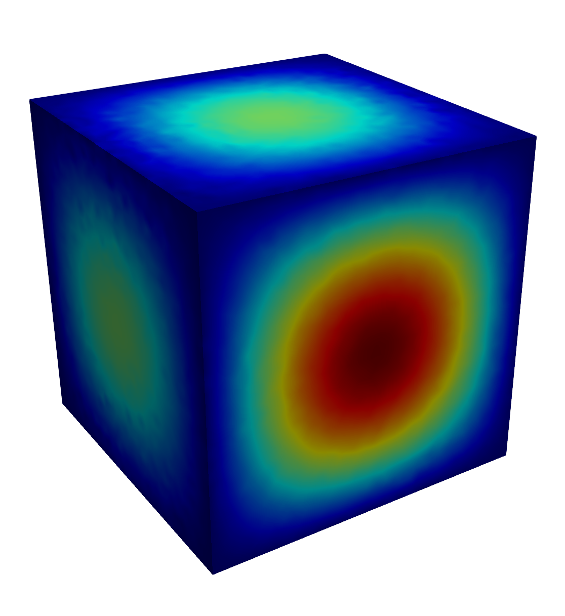
../_images/ex_maxwell3dN1_app.png — Fig. 9 Module of the solution of the Maxwell 3D problem using Nedelec first family elements#

Alternatively, the interpolate function provides the interpolation of $E$ on nodes of a P1 approximation.

On the next figure, the convergence curve shows a rate convergence of $L^{2}$ error in $h^{1.3}$ :

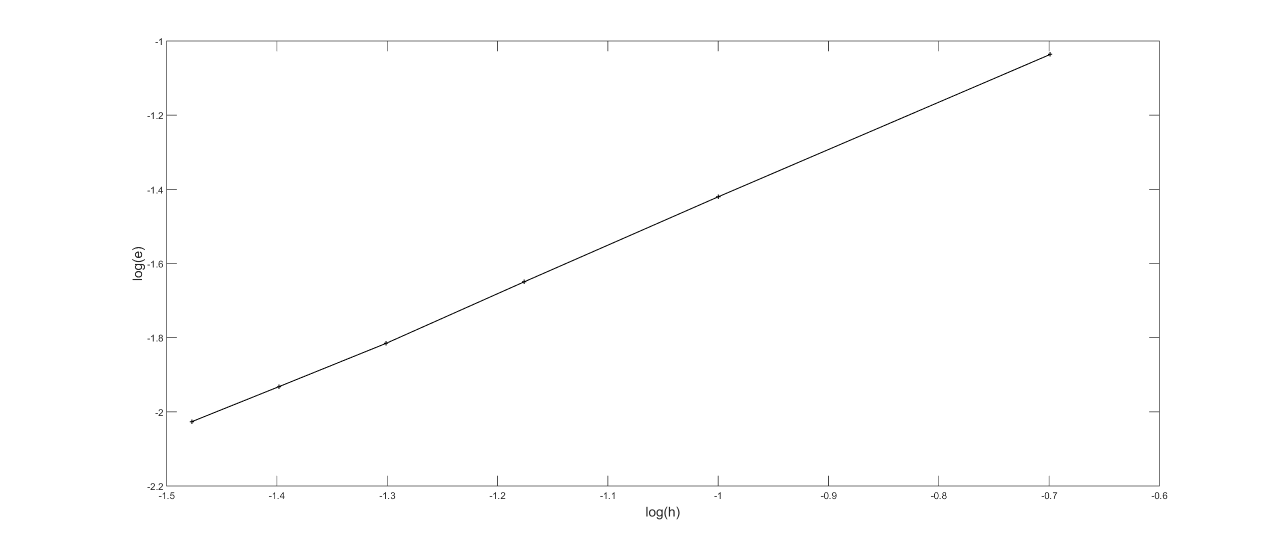
../_images/Nedelec3d_convergence.png — Fig. 10 $L^{2}$ errors versus the step $h$ for first order Nedelec first family approximation#