Solving wave equation with Leap-frog scheme#

Keywords: PDE:Wave Method:FEM FE:Lagrange Condition:Dirichlet Solver:Direct

So far, only the harmonic problems were considered. Time problem may also be solved using XLiFE++. But there is no specific tools dedicated to. Users have to implement the time loop related to the finite difference time scheme they choose.

As an example, consider the wave equation:

\begin{array}{r} {\begin{cases} \frac{\partial^{2} u}{\partial t^{2}} - c^{2} Δ u = f & in Ω \times] 0, T [ \\ \frac{\partial u}{\partial n} = 0 & in \partial Ω \times] 0, T [ \\ u (x, 0) = \frac{\partial u}{\partial t} (x, 0) = 0 & in Ω \end{cases} \end{array}

Using classical leap-frog scheme with time discretization $t^{n} = n Δ t$ , leads to ( $u^{n}$ approximates $u (x, t^{n})$ ):

\begin{array}{r} {\begin{cases} u^{n + 1} = 2 u^{n} - u^{n - 1} + (c Δ t)^{2} Δ u^{n} + (Δ t)^{2} f^{n} & in Ω, \forall n > 1 \\ \frac{\partial u^{n}}{\partial n} = 0 & in \partial Ω, \forall n > 1 \\ u^{0} = u^{1} = 0 & in Ω \end{cases} \end{array}

or, in variational form, $\forall v \in V = H^{1} (Ω)$ :

\begin{array}{r} {\begin{cases} \int_{Ω} u^{n + 1} v = 2 \int_{Ω} u^{n} v - \int_{Ω} u^{n - 1} v - (c Δ t)^{2} \int_{Ω} \nabla u^{n} . \nabla v + (Δ t)^{2} \int_{Ω} f^{n} v \forall n > 1 \\ u^{0} = u^{1} = 0 in Ω \end{cases} \end{array}

When approximating space $V$ by a finite dimension space $V_{h}$ with basis $(w_{i})_{i = 1, p}$ , the variational formulation is reinterpreted in terms of matrices and vectors as follows:

\begin{array}{r} {\begin{cases} U^{n + 1} = 2 U^{n} - U^{n - 1} - M^{- 1} ((c Δ t)^{2} K U^{n} - (Δ t)^{2} F^{n}) \forall n > 1 \\ U^{0} = U^{1} = 0 in Ω \end{cases} \end{array}

where

M_{i j} = \int_{Ω} w_{i} w_{j}, K_{i j} = \int_{Ω} \nabla w_{i} . \nabla w_{j}, (F^{n})_{i} = \int_{Ω} f^{n} w_{i} .

The XLiFE++ implementation of this scheme on the unity square when using P1 Lagrange interpolation looks like ( $f (x, t) = h (t) g (x)$ ):

#include "xlife++.h"
using namespace xlifepp;

Real g(const Point& P, Parameters& pa = defaultParameters)
{
  Real d=P.distance(Point(0.5, 0.5));
  Real R= 0.02;        // source radius
  Real amp= 1./(pi_*R*R); // source amplitude (constant power)
  if (d<=0.02) return amp; else return 0.;
}

Real h(const Real& t)
{
  Real a=10000, t0=0.04 ; //gaussian slope and center
  return exp(-a*(t-t0)*(t-t0));
}

int main(int argc, char** argv)
{
  init(argc, argv, _lang=en);
  // create a mesh and domain omega
  SquareGeo sq(_origin=Point(0., 0.), _length=1, _nnodes=70);
  Mesh mesh2d(sq, _shape=triangle, _generator=structured);
  Domain omega=mesh2d.domain("Omega");
  // create interpolation
  Space V(_domain=omega, _interpolation=P1, _name="V");
  Unknown u(V, _name="u");
  TestFunction v(u, _name="v");
  // define FE terms
  TermMatrix A(intg(omega, grad(u)|grad(v)), _name="A"), M(intg(omega, u*v), _name="M");
  TermVector G(intg(omega, g*v), _name="G");
  TermMatrix L; ldltFactorize(M, L);
  // leap-frog scheme
  Real c=1, dt=0.004, dt2=dt*dt, cdt2=c*c*dt2;
  Number nbt=200;
  TermVectors U(nbt);  // to store solution at t=ndt
  TermVector zeros(u, omega, 0.);  U(1)=zeros;  U(2)=zeros;
  Real t=dt;
  for (Number n=2; n<nbt; n++, t+=dt)
  {
    U(n+1)=2.*U(n)-U(n-1)-factSolve(L, cdt2*(A*U(n))-dt2*h(t)*G);
  }
  saveToFile("U", U, vtu);
  return 0;
}

Note the very simple syntax taken into account the leap-frog scheme. The following figure represents the solution at different instants for a constant source localized in disk with center $(0.5, 0.5)$ , radius $R = 0.02$ and time excitation that is a Gaussian function. For chosen parameter $d t = 0.04$ , the leap-frog scheme is stable (it satisfies the CFL condition) but dispersion effects obviously appear.

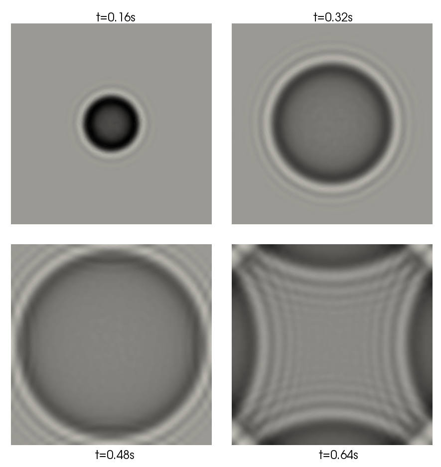
../_images/wave2d.png — Fig. 12 Solution of the wave equation at different instants for a constant source localized in disk with center $(0.5, 0.5)$ #

Using Lagrange FE with Gauss-Lobatto points with a Gauss-Lobatto quadrature defining on same points as FE dofs, leads to a diagonal mass matrix and better peformance:

Rectangle rect(_xmin=-1, _xmax=1, _ymin=-1, _ymax=1, _hsteps=0.1, _domain_name="Omega");
Mesh meshR(rect);
Domain omega=meshR.domain("Omega");
Number k=2;
Space V(_domain=omega,_FE_type=Lagrange,_FE_subtype=GaussLobattoPoints,_order=k,_name="V");
Unknown u(V, _name="u"); TestFunction v(u, _name="v");
BilinearForm a = intg(omega, grad(u)|grad(v)),
             m = intg(omega, u * v, _diagonal);   // diagonal matrix
TermMatrix A(a, _name="A"), M(m, _name="M");
G = TermVector(intg(omega,g*v), _name="G");
TermMatrix L = inverse(M);             //inverse of a diagonal matrix
Real c=1, dt=0.004, dt2=dt*dt, cdt2=c*c*dt2, t=dt;
Number nbt=200;
TermVector zeros(u, omega, 0.);
TermVectors U(nbt);  U(1)=zeros;  U(2)=zeros;
for (Number n=2; n<nbt; n++, t+=dt)
   U(n+1)=2.*U(n)-U(n-1)-L*(cdt2*(A*U(n))-dt2*h(t)*G);

../_images/wave2d_Lobatto.png — Fig. 13 Solution of the wave equation at $t = 0.8$ for different approximations (P1, P2, Q1, Q2, Q1 Lobatto, Q2 Lobatto)#

The following table gives the computation times of different part of the code :

preparation (computation of FE matrices and vectors, factorization or inversion of the mass matrix )
in loop, linear combination of vectors involving a matrix product
in loop, solving a factorized linear system or product by a diagonal matrix

Table 1 computation times versus approximation#
	nb dl	nb t	preparation	combination	solving	by step	total
$P1$	$10200$	$400$	$0.476$	$0.341$	$0.992$	$3.32 10^{- 3}$	$1.81$
$Q1$	$10200$	$400$	$0.318$	$0.346$	$1.03$	$3.42 10^{- 3}$	$1.69$
$Q1 Lobatto$	$10200$	$400$	$0.237$	$0.183$	$0.065$	$6.18 10^{- 4}$	$\underset{―}{0.485}$
$P2$	$40400$	$800$	$2.03$	$1.65$	$15.3$	$2.12 10^{- 2}$	$19$
$Q2$	$40400$	$800$	$2.44$	$1.71$	$15.9$	$2.20 10^{- 2}$	$20.1$
$Q2 Lobatto$	$40400$	$800$	$0.602$	$1.463$	$0.299$	$2.2 10^{- 3}$	$\underset{―}{2.36}$

Obvously, Lagrange-Lobatto FE is faster : four times faster at order 1, eight times faster at order 2. The gain comes from replacing the resolution of a factorized linear system by a product of a diagonal matrix (50 times faster at order 2). The gain becomes greater and greater as the order increases!

Caution

Lagrange-Lobatto FE are only available for segment, quadrangle and hexaedron shape. To get diagonal matrix, specify the key _diagonal when defining the bilinear form. This key is only available for Lagrange-Lobatto FE.