2D Laplace Problem with Discontinuous Galerkin method and Dirichlet condition

Keywords: PDE:Laplace Method:DG FE:Lagrange Condition:Dirichlet Solver:Direct

Consider the Laplace problem with homogeneous Dirichlet condition:

\[\begin{split}\begin{cases} -\Delta u = f & \mathrm{\;in\;}\Omega \\ u=0 & \mathrm{\;on\;}\partial \Omega \end{cases}\end{split}\]

Consider a discontinuous Galerkin space \(V_h\), e.g. discontinuous P1-Lagrange space and let introduce the IP (Interior Penalty) formulation:

\[\begin{split}\left| \begin{array}{l} \mathrm{find\;} u_h\in V_h \mathrm{\;such\;that\;} \\ \displaystyle \int_\Omega \nabla_hu_h.\nabla_hv -\int_\Gamma \big\{\nabla_hu_h.n\big\}\,\big[v\big] -\int_\Gamma \big[u_h\big]\,\big\{\nabla_hv.n\big\} +\int_\Gamma\mu \big[u_h\big]\,\big[v\big] =\int_\Omega f\,v\quad \forall v\in V_h. \end{array} \right.\end{split}\]

where \(\Omega=\bigcup T_\ell\), \(\Gamma =\bigcup \partial T_\ell\) (the set of all sides of mesh elements) and, \(S_{k,\ell}\) denoting the side shared by the elements \(T_k\) and \(T_\ell\):

\[\big\{v\big\}_{|S_{k\ell}}=\dfrac{1}{2}\left((v_{|T_k})_{|S_{k\ell}} + (v_{|T_\ell})_{|S_{k\ell}} \right )\quad \big[v\big]_{|S_{k\ell}}=\left((v_{|T_k})_{|S_{k\ell}} - (v_{|T_\ell})_{|S_{k\ell}} \right ).\]

For a non-shared side \(S_k\), we set

\[\big\{v\big\}_{|S_{k}}=\big[v\big]_{|S_{k}}=(v_{|T_k})_{|S_{k}}.\]

The operators \(\{.\}\) and \([.]\) are implemented in XLiFE++ as mean() and jump() operators. The normal vector \(n\) is chosen as the outward normal from \(T_k\) on side \(S_{k\ell}\); in practice outward from the “first” parent element of the side. \(\mu\) is a penalty function usually chosen to be proportional to the inverse of the measure of the side \(S_{k\ell}\). Note that the Dirichlet boundary condition is a natural condition in this formulation.

To deal with a such formulation, the following objects have to be constructed from a geometrical domain, say omega:

• a FE space specifying \(L2\) conformity (discontinuous space) defined on omega

• the geometrical domain gamma of sides of omega using the function sides()

• the bilinear form related to IP formulation and involving mean() and jump() operators

The XLiFE++ implementation of this problem using discontinuous P1-Lagrange is the following:

#include "xlife++.h"
using namespace xlifepp;

Real uex(const Point& p, Parameters& pars=defaultParameters)
{return sin(pi_*p(1))*sin(pi_*p(2));}
Real f(const Point& p, Parameters& pars=defaultParameters)
{return 2*pi_*pi_*sin(pi_*p(1))*sin(pi_*p(2));}
Real fmu(const Point& p, Parameters& pars=defaultParameters)
{GeomElement* gelt=getElementP();
 if(gelt!=0) return 1/gelt->measure();
 return 0.;
}

int main(int argc, char** argv)
{
  init(argc, argv, _lang=en); // mandatory initialization of xlifepp
  // create mesh and geometrical domains
  Rectangle R(_origin=Point(0.,0.),_xlength=1., _ylength=1.,_nnodes=31,_domain_name="Omega");
  Mesh mR(R, _shape=triangle, _generator=structured, _split_direction=alternate);
  Domain omega=mR.domain("Omega");
  Domain gamma=sides(omega);  // create domain of sides
  // create discontinuous P1-Lagrange space
  Space V(_domain=omega, _FE_type=Lagrange, _order=1, _Sobolev_type=L2, _name="V");
  Unknown u(V, _name="u"); TestFunction v(u, _name="v");
  // create bilinear form and TermMatrix
  Function mu(fmu); mu.require("element");
  BilinearForm a=intg(omega,grad(u)|grad(v))-intg(gamma,mean(grad(u)|_n)*jump(v))
                -intg(gamma,jump(u)*mean(grad(v)|_n))+intg(gamma,mu*jump(u)*jump(v));
  TermMatrix A(a, _name="A");
  // create the right hand side an solve the linear system
  TermVector F(intg(omega,f*v), _name="F");
  TermVector U=directSolve(A,F);
  saveToFile("U", U, _format=vtu);
  // compute L2 error
  TermMatrix M(intg(omega,u*v), _name="M");
  TermVector Uex(u, omega, uex);
  TermVector E=U-Uex;
  theCout<<"  IP : |U-uex|L2 = "<<sqrt(M*E|E)<<eol;
  return 0;
}

The \(L^2\) error is about \(0.00317\) for 5400 DoFs. Using Paraview with the Warp by scalar filter that produces elevation, the approximated field \(u\) looks like:

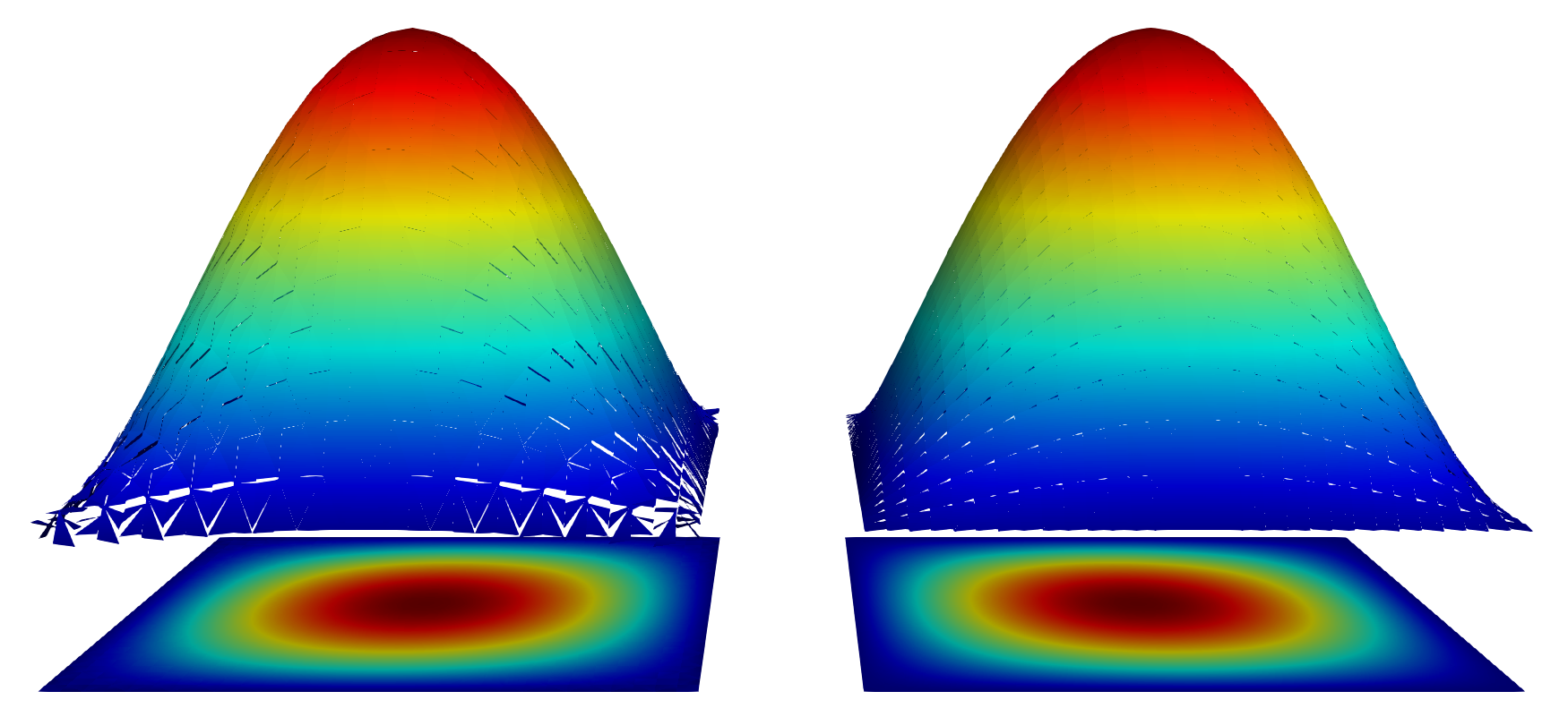
Fig. 4 Solution of the 2D Dirichlet problem on the unit square \([0,1]^2\) with discontinuous P1-Lagrange elements, IP formulation (left) and NIPG formulation (right)

It can be noticed that the field is discontinuous and major errors is located on the corners. NIPG formulation is another penalty method corresponding to the bilinear form:

\[\displaystyle \int_\Omega \nabla_hu_h.\nabla_hv -\int_\Gamma \big\{\nabla_hu_h.n\big\}\,\big[v\big] +\int_\Gamma \big[u_h\big]\,\big\{\nabla_hv.n\big\} +\int_\Gamma\mu \big[u_h\big]\,\big[v\big]\]

that is close to the IP formulation but non-symmetric. For NIPG, the \(L^2\) error is weaker (about \(0.00141\)) and the solution is less polluted at the corners.