3D Maxwell problem using EFIE#

Keywords: PDE:Maxwell Method:BEM FE:Lagrange FE:RaviartThomas Solver:Direct

Solving diffraction of an electromagnetic plane wave on a obstacle using BEM is more intricate. Indeed, it is a vector problem and it involves Raviart-Thomas elements. We show how XLiFE++ can deal easily with.

Let $Γ$ be the boundary of a bounded domain $Ω$ of $R^{3}$ , we want to solve the Maxwell problem on the exterior domain $Ω_{e}$ :

\begin{array}{r} {\begin{cases} curl E - i k H = 0 & in Ω_{e} \\ curl H + i k E = 0 & in Ω_{e} \\ E \times n = 0 & on Γ \\ lim_{| x | \to \infty} ((H - H_{i n c}) \times \frac{x}{| x |} - (E - E_{i n c})) = 0 & (Silver - Muller condition) \end{cases} \end{array}

where $(E_{i n c}, H_{i n c})$ is an incident field (a solution of Maxwell equation in free space), for instance a plane wave.

The EFIE (Electric Field Integral Equation) consists in finding the potential $J$ in the space

H_{div} (Γ) = {V \in L^{2} (Γ)^{3}, V \cdot n = 0, {div}_{Γ} V \in L^{2} (Γ)}

such that:

\forall V \in H_{div} (Γ), k \int_{Γ} \int_{Γ} J (y) * G (x, y) * V (x) - \frac{1}{k} \int_{Γ} \int_{Γ} \div_{Γ} J (y) * G (x, y) * \div_{Γ} V (x) = - \int_{Γ} E_{i n c} \cdot V

where $G$ is the Green function related to the Helmholtz 3D problem in free space.

This equation has a unique solution, except for a discrete set of wavenumbers corresponding to the resonance frequencies of the cavity $Ω$ .

Using the Stratton-Chu representation formula, the scattered electric field may be reconstructed in $Ω_{e}$ :

E (x) = E_{i n c} (x) + \frac{1}{k} \int_{Γ} \nabla_{x} G (x, y) {div}_{Γ} J (y) + k \int_{Γ} G (x, y) * J (y) .

This problem is implemented in XLiFE++ as follows:

#include "xlife++.h"
using namespace xlifepp;
Vector<complex_t> data_incField(const Point& P, Parameters& pars)
{
  Vector<real_t> incPol(3, 0.); incPol(1)=1.; Point incDir(0., 0., 1.) ;
  Real k = pars("k");
  return  incPol * exp(i_*k * dot(P, incDir));
}

Vector<complex_t> uinc(const Point& P, Parameters& pars)
{
  Vector<real_t> incPol(3, 0.); incPol(1)=1.; Point incDir(0., 0., 1.) ;
  Real k = pars("k");
  return  incPol*exp(i_*k * dot(P, incDir));
}

int main(int argc, char** argv)
{
  init(argc, argv, _lang=en);
  // define parameters and functions
  Real k= 1, R=1.; Parameters pars;
  pars << Parameter(k, "k") << Parameter(R, "radius");
  Kernel H = Helmholtz3dKernel(pars);          // load Helmholtz3D kernel
  Function Einc(data_incField, pars);          // define right hand side 
  Function Uex(scatteredFieldMaxwellExn, pars);
  // meshing the unit sphere
  Number npa=15; Point O(0, 0, 0);                          
  Sphere sphere(_center=O, _radius=R, _nnodes=npa, _domain_name="Gamma");
  Mesh meshSh(sphere, _shape=triangle, _generator=gmsh);
  Domain Gamma = meshSh.domain("Gamma");
  // define FE-RT1 space and unknown
  Space V_h(_domain=Gamma, _interpolation=RT_1, _name="Vh");
  Unknown U(V_h, _name="U"); TestFunction V(U, _name="V");
  // compute BEM system and solve it
  IntegrationMethods ims(_method=SauterSchwabIM, _order=4, _bound=0.,
                         _quad=defaultQuadrature, _order=5, _bound=2.,
                         _quad=defaultQuadrature, _order=3);
  BilinearForm auv = k*intg(Gamma, Gamma, U*H|V, ims)
                   -(1./k)*intg(Gamma, Gamma, div(U)*H*div(V), ims);
  TermMatrix A(auv, _name="A");
  TermVector B(-intg(Gamma, Einc|V));
  TermVector J = directSolve(A, B);
  // get P1 representation of solution and export it to vtu file
  Space L_h(_domain=Gamma, _interpolation=P1, _name="Lh");
  Unknown U3(L_h, _name="U3", _dim=3); TestFunction V3(U3, _name="V3");
  TermVector JP1=projection(J, L_h, 3, _L2Projector);
  saveToFile("JP1", JP1(U3[1]), vtu);
  // integral representation on y=0 plane (excluding sphere), using P1 nodes
  Number npp=30, npc=5;
  Square sqx(_center=O, _length=20., _nnodes=npp, _domain_name="Omega");
  Disk dx(_center=O, _radius=1.2*R, _nnodes=npc);
  Mesh mx0(sqx-dx, _shape=triangle, _generator=gmsh);
  mx0.rotate3d(1., 0., 0., pi_/2);
  Domain py0 = mx0.domain("Omega");
  Space Vy0(_domain=py0, _interpolation=P1, _name="Vy0", _notOptimizeNumbering);
  Unknown W(Vy0, _name="W", _dim=3);
  IntegrationMethods im(_quad=defaultQuadrature, _order=10, _bound=1., _quad=defaultQuadrature, _order=5);
  TermVector Uext=(1./k)*integralRepresentation(W, py0, intg(Gamma, grad_x(H)*div(U), _method=im), J)
                  + k*integralRepresentation(W, py0, intg(Gamma, H*U, _method=im), J);
  saveToFile("Uext", Uext, _format=vtu);
  // build exact solution, export to vtu file and compute error
  TermVector Uexa(W, py0, Uex);
  saveToFile("Uexa", Uexa, _format=vtu);
  TermMatrix M(intg(py0, W|W));
  TermVector E=Uext-Uexa;
  theCout << "L2 error = " << sqrt(real(M*E|E)) << eol;
  return 0;
}

In order to build an approximated space of $H_{div} (Γ)$ we use the Raviart-Thomas element of order 1.

As the integrals involved in bilinear form are singular, we use here the Sauter-Schwab method to compute them when two triangles are adjacent, a quadrature method of order 5 if the two triangles are close ( $0 < d (T 1, T 2) < 2 h$ ) and a quadrature method of order 3 when the two triangles are far ( $d (T 1, T 2) >= 2 h$ ).

Note that the unknowns in RT approximation are the normal fluxes on the edge of the triangulation. In order to plot the potential $J$ , we have to move to a P1 representation, say $\tilde{J}$ . This can be done using a L2 projection from $H_{div} (Γ)$ to $L^{2} (Γ)$ :

\forall V \in L^{2} (Γ), \int_{Γ} \tilde{J} \cdot V = \int_{Γ} J \cdot V

This is what is done by the XLiFE++ function projection.

We obtain the following potential:

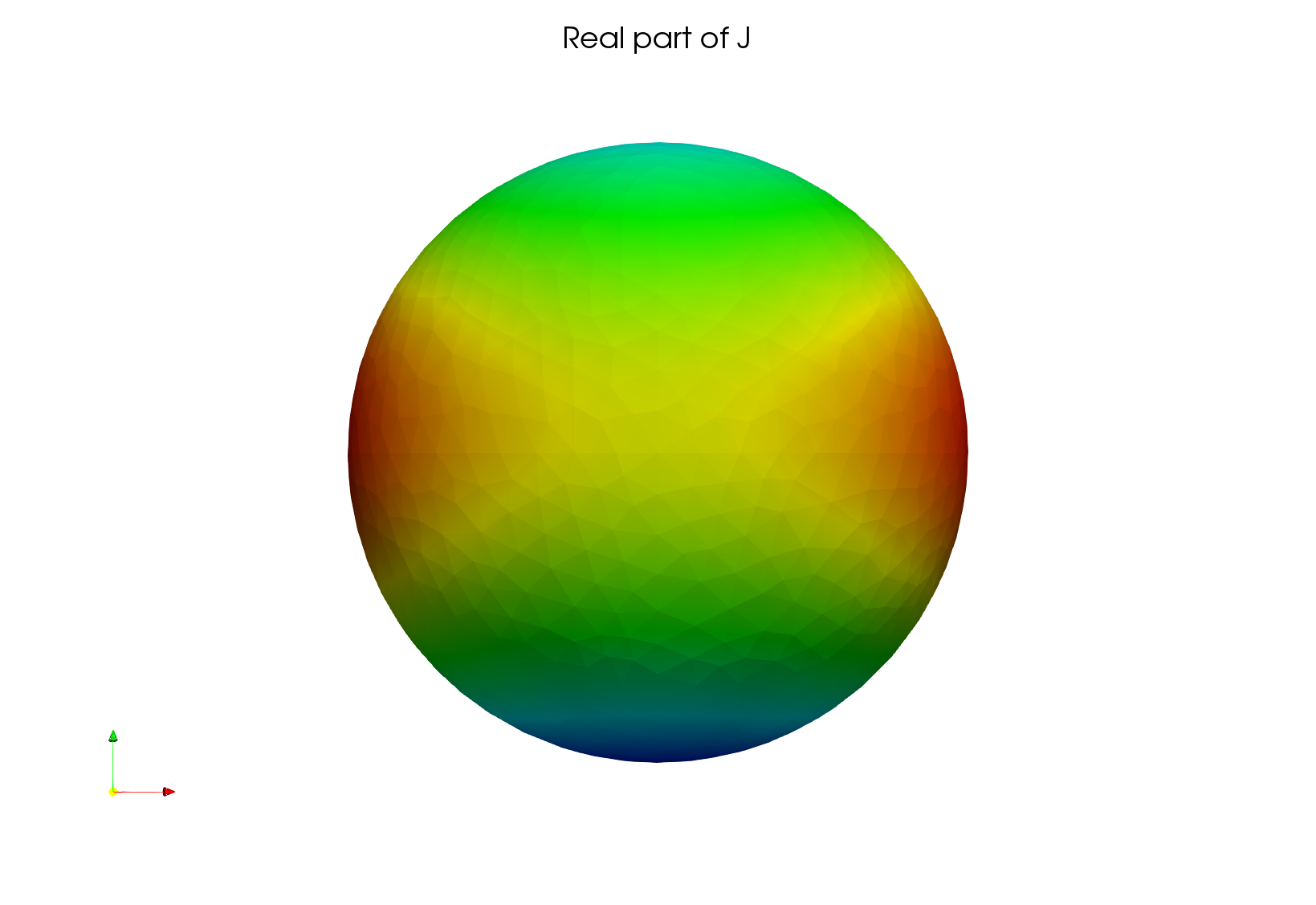
../_images/J_real.png — Fig. 28 3D Maxwell problem on the unit sphere, using EFIE, potential#

On the following figures, we show the approximated electric field and the exact electric field. The component $E_{y}$ is not shown because it is zero.

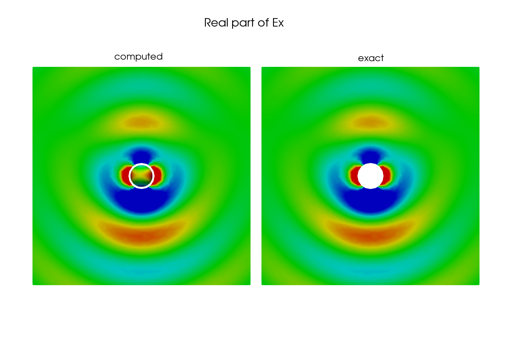
../_images/Ex_real.png — Fig. 29 3D Maxwell problem on the unit sphere, using EFIE, x component#

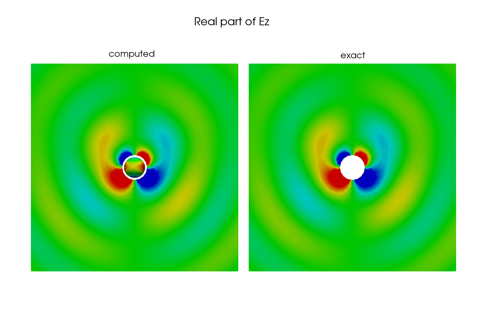
../_images/Ez_real.png — Fig. 30 3D Maxwell problem on the unit sphere, using EFIE, y component#