2D Stokes problem#

Keywords: PDE:Stokes Method:FEM FE:CrouzeixRaviart FE:TaylorHood Condition:Dirichlet Solver:Direct

We consider the problem of a flow entrained in a cavity, say $Ω =] 0, 1 [\times] 0, 1 [$ :

\begin{array}{r} {\begin{cases} - ν △ u + \nabla p = f & in Ω \\ div u = 0 & in Ω \\ u = g & on Σ = {0} \times] 0, 1 [ \\ u = 0 & on Γ = \partial Ω ∖ Σ \end{cases} \end{array}

with $f \in L^{2} (Ω)$ and $g = (0, v_{0}), v_{0} \in H_{00}^{\frac{1}{2}} (Σ)$ . Note that $g | n = 0$ .

This problem has the following variational formulation: find $(u, p) \in H^{1} (Ω)^{2} \times L_{0}^{2} (Ω)$ such that for all $(v, p) \in H_{0}^{1} (Ω)^{2} \times L_{0}^{2} (Ω)$ :

\begin{array}{r} {\begin{cases} ν \int_{Ω} \nabla u : \nabla v - \int_{Ω} p div v - \int_{Ω} div u q = \int_{Ω} f \cdot v \\ u = g on Σ and u = 0 on Γ \end{cases} \end{array}

The following XLiFE++ implementation of this problem solves the 2D Stokes problem using different couples of approximation for the velocity $v$ and the pressure $p$ : (P2, P0), (P2, P1), (CR, P0); CR corresponds to a P1 Crouzeix-Raviart finite element approximation leading to a non-conforming approximation of $H^{1}$ . Note that the (P1, P0) approximation is not working because of dof locking.

#include "xlife++.h"
using namespace xlifepp;
using namespace std;

Vector<Real> g(const Point& p, Parameters& pa = defaultParameters)
{
    Vector<Real> r(2,0.);
    r(2)=1.;
    return r;
}

int main(int argc, char** argv)
{
  init(_lang=en); // mandatory initialization of xlifepp
  verboseLevel(1);
  //geometry data
  Square sq(_origin=Point(0.,0.),_length=1., _nnodes=30, _domain_name="Omega",
            _side_names=Strings("Gamma","Gamma", "Gamma", "Sigma"));
  Mesh mesh(sq, _shape=triangle);
  Domain Omega=mesh.domain("Omega");
  Domain Sigma=mesh.domain("Sigma");
  Domain Gamma=mesh.domain("Gamma");
  // solve Stokes 2D for several approximations
  list<pair<InterpolationType,InterpolationType>> pint={{P0,P2},{P1,P2},{P0,CR}};
  for (auto ps:pint)
  {
    Space H1(_domain=Omega,_interpolation=ps.second,_name="H1");
    Unknown u(H1,_name="u",_dim=2); TestFunction v(u,_name="v");
    Space L2(_domain=Omega,_interpolation=ps.first,_name="L2");
    Unknown p(L2,_name="p"); TestFunction q(p,_name="q");
    BilinearForm a = intg(Omega,grad(u)%grad(v))-intg(Omega,p*div(v))-intg(Omega,div(u)*q);
    EssentialConditions ecs = (u|Gamma = 0) & (u | Sigma = g) & (intg(Omega,p)=0);
    TermMatrix A(a,ecs,_name="A");
    TermVector b(u,Omega,0.,_name="b");
    TermVector X=directSolve(A,b);
    String filename=fileNameFromComponents("u", words("interpolation",ps.first)+"_"+words("interpolation",ps.second), "vtu");
    saveToFile(filename, X(p));
    if (ps.second==_CR)
    {
      Space V1(_domain=Omega,_interpolation=P1, _name="V1");
      TermVector u1=projection(X(u),V1,2);
      saveToFile(filename, u1, _data_name="u1");
    }
    else saveToFile(filename, X(u));
  }
  return 0;
}

Using Paraview with the Glyph filter that represents 2D vectors with arrows, we get the following pictures:

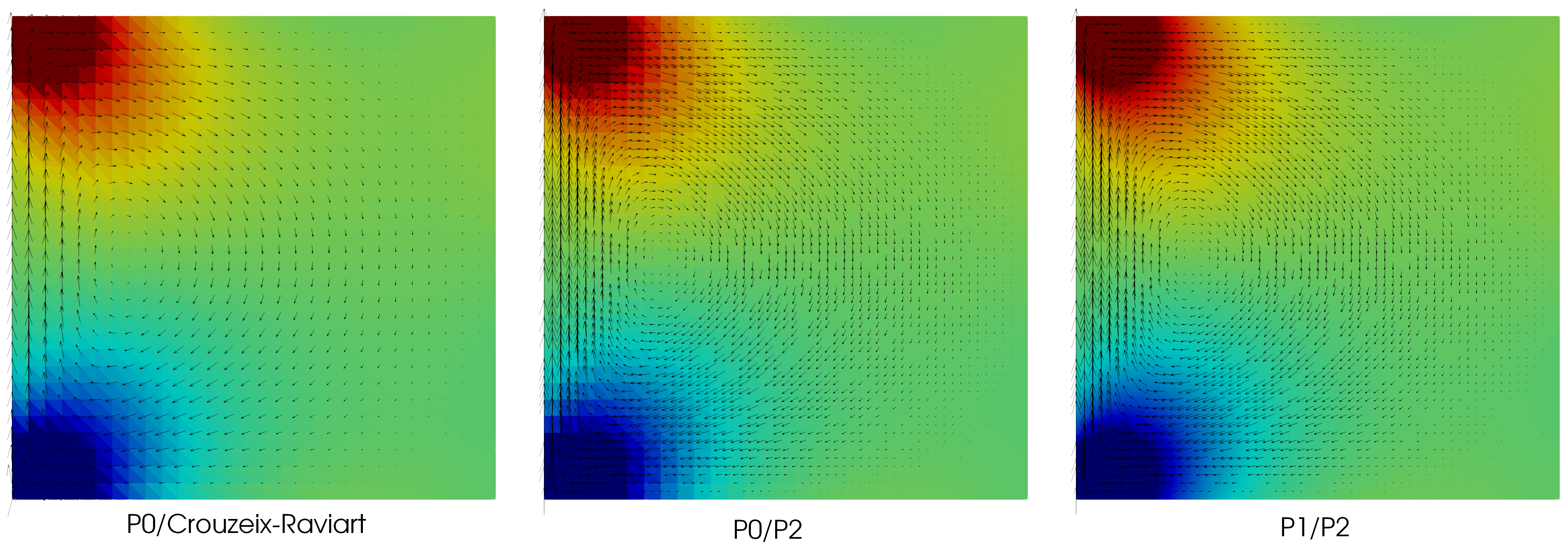
Fig. 11 Solution of the 2D Stokes problem using different approximations#

Note that to approximate the space $L_{0}^{2} (Ω)$ , an essential condition of the zero mean type of pressure p has been used. Such a condition is quite costly because it interacts with all the pressure dofs. If we remove it, the matrix becomes singular (the pressure being defined to within a constant) and direct solvers fail. But iterative solvers do converge to the right velocity, and pressure to the right constant, determined by the initial guess of the iterative solver !

Note also that, when using Crouzeix-Raviart element, in order to visualize the velocity, it is required to project the CR solution in a standard Lagrange finite element space (here $P_{1}$ ).