3D Helmholtz problem using single layer potential integral equation

Keywords: PDE:Helmholtz Method:BEM FE:Lagrange Solver:Direct

XLiFE++ is also able to deal with integral equation. This example illustrates the computation of the acoustic scattering by a sphere:

\[\begin{split}\begin{cases} \displaystyle \Delta u + k^2 u = 0 & \mathrm{\;in\;}\Omega=\mathbb{R}^3/B(0,R) \\ \displaystyle u=-u_{inc} & \mathrm{\;on\;} S \end{cases}\end{split}\]

Using single layer potential leads to the integral equation:

\[\int_S G(x,y)p(y)dy = -u_{inc}\ \ \ \mathrm{\;on\;}S\]

where \(G\) is the Green function of the Helmholtz equation:

\[G(x,y)=\dfrac{e^{ik|x-y|}}{4\pi|x-y|}.\]

We deal with the variational formulation in \(V=H^{\frac{1}{2}}(S)\):

\[\mathrm{find\;} p \in V \mathrm{\;such\;that\;} \int_S \int_S p(y) G(x,y) \bar{q}(x) dx dy = -\int_S u_{inc} \bar{q} \quad \forall q\in V.\]

The solution \(u\) is got from potential \(p\) using the integral representation:

\[u(x)=\int_S G(x,y) p(y)dy.\]

This example has been implemented in XLiFE++ using a \(P^0\) Lagrange interpolation:

#include "xlife++.h"
using namespace xlifepp;

// incident plane wave
Complex uinc(const Point& p, Parameters& pa = defaultParameters)
{
  Real kx=pa("kx"), ky=pa("ky"), kz=pa("kz");
  Real kp=kx*p(1)+ky*p(2)+kz*p(3);
  return exp(i_*kp);
}

int main(int argc, char** argv)
{
  init(argc, argv, _lang=en); // mandatory initialization of xlifepp

  // define parameters and functions
  Parameters pars;
  pars << Parameter(1., "k");                // wave number k
  pars << Parameter(1., "kx") << Parameter(0., "ky") << Parameter(0., "kz"); // kx, ky, kz
  pars << Parameter(1., "radius");           // sphere radius
  Kernel G = Helmholtz3dKernel(pars);     // load Helmholtz3D kernel
  Function finc(uinc, pars);              // define right hand side function
  Function scatSol(scatteredFieldSphereDirichlet, pars);  // exact solution

  // meshing the unit sphere
  Number npa=16;      // nb of points by diameter of sphere
  Sphere sp(_center=Point(0, 0, 0), _radius=1, _nnodes=npa, _domain_name="sphere");
  Mesh mS(sp, _shape=triangle, _generator=gmsh);
  Domain sphere = mS.domain("sphere");

  // Lagrange P0 space and unknown
  Space V0(_domain=sphere, _interpolation=P0, _name="V0", _notOptimizeNumbering);
  Unknown u0(V0, _name="u0");
  TestFunction v0(u0, _name="v0");
  IntegrationMethods ims(_method=SauterSchwab, _order=3, _quad=symmetricalGauss, _order=3);
  BilinearForm blf0=intg(sphere, sphere, u0*G*v0, _method=ims);
  LinearForm fv0 = -intg(sphere, finc*v0);

  // compute matrix and right hand side and solve system
  TermMatrix A0(blf0, _storage=denseDual, _name="A0");
  TermVector B0(fv0, _name="B0");
  TermVector U0 = directSolve(A0, B0);

  // integral representation on x plane (far from sphere), using P1 nodes
  Number npp=20, npc=8*npp/10;
  Real xm=4., eps=0.0001;
  Point C1(0., -xm, -xm), C2(0., xm, -xm), C3(0., -xm, xm);
  Rectangle recx(_v1=C1, _v2=C2, _v4=C3, _nnodes=npp);
  Disk dx(_center=Point(0., 0., 0.), _v1=Point(0., 1.25, 0.), _v2=Point(0., 0., 1.25), _nnodes=npc);
  Mesh mx0(recx-dx, _shape=triangle, _generator=gmsh);
  Domain planx0 = mx0.domain("Omega");
  Space Wx(_domain=planx0, _interpolation=P1, _name="Wx", _notOptimizeNumbering);
  Unknown wx(Wx, _name="wx");
  TermVector U0x0=integralRepresentation(wx, planx0, intg(sphere, G*u0), U0);
  TermMatrix Mx0(intg(planx0, wx*wx), _name="Mx0");

  // compare to exact solution
  TermVector solx0(wx, planx0, scatSol);
  TermVector ec0x0=U0x0 - solx0;
  theCout << " L2 error on x=0 plane : " << sqrt(abs((Mx0*ec0x0) | ec0x0)) << eol;

  // export solution to file
  saveToFile("U0", U0, _format=vtu);
  saveToFile("U0x0", U0x0, _format=vtu);
  return 0;
}

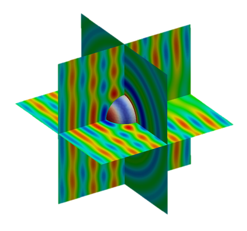
Fig. 23 Solution of the 3D Helmholtz problem using single layer BEM on the unit sphere