2D Laplace problem with Dirichlet condition#

Keywords: PDE:Laplace Method:FEM FE:Lagrange Condition:Dirichlet Solver:Direct

Let us consider now the case of non-homogeneous Dirichlet condition on the boundaries $x = 0$ ( $Σ^{-}$ ) and $x = 1$ ( $Σ^{+}$ ):

u = 1 on Σ^{-} \cup Σ^{+} .

The variational formulation is now ( $a = 0$ )

\begin{array}{r} | \begin{array}{c} find u \in V = {v \in L^{2} (Ω), \nabla v \in (L^{2} (Ω))^{2}} such that \\ \begin{aligned} \int_{Ω} \nabla u . \nabla v = \int_{Ω} f v & \forall v \in V, v = 0 on Σ^{-} \cup Σ^{+} \\ u = 1 & on Σ^{-} \cup Σ^{+} \end{aligned} \end{array} \end{array}

Its approximation by P1 Lagrange finite element is implemented in XLiFE++ as follows:

#include "xlife++.h"
using namespace xlifepp;

Real f(const Point& P, Parameters& pa = defaultParameters)
{return -8.;}

int main(int argc, char** argv)
{
  init(argc, argv, _lang=en); // mandatory initialization of xlifepp

  // create mesh of square
  Strings sn("y=0", "x=1", "y=1", "x=0");
  SquareGeo sq(_origin=Point(0., 0.), _length=1, _nnodes=20, _domain_name="Omega", _side_names=sn);
  Mesh mesh2d(sq, _shape=triangle, _generator=structured);
  Domain omega=mesh2d.domain("Omega");
  Domain sigmaM=mesh2d.domain("x=0"), sigmaP=mesh2d.domain("x=1");

  // create interpolation
  Space V(_domain=omega, _interpolation=P1, _name="V");
  Unknown u(V, _name="u");
  TestFunction v(u, _name="v");

  // create bilinear form, linear form and their algebraic representation
  BilinearForm auv=intg(omega, grad(u)|grad(v));
  LinearForm fv=intg(omega, f*v);
  EssentialConditions ecs= (u|sigmaM = 1) & (u|sigmaP = 1);
  TermMatrix A(auv, ecs, _name="A");
  TermVector B(fv, _name="B");

  // solve linear system AX=B
  TermVector U=directSolve(A, B);
  saveToFile("U_LD", U, _format=vtu);
  return 0;
}

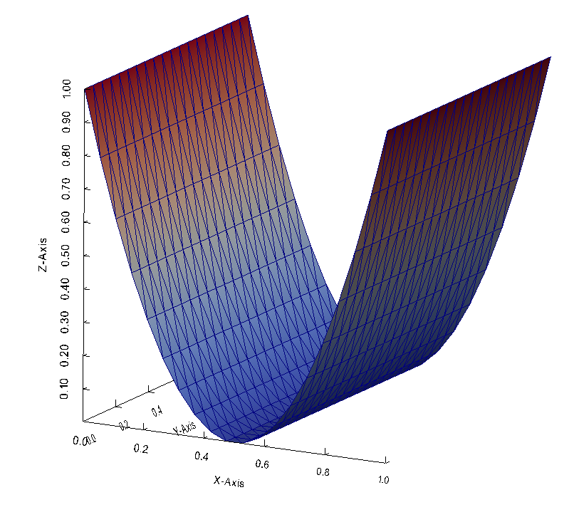
../_images/ex_2d_dirichlet.png — Fig. 6 Solution of the Laplace 2D problem with Dirichlet condition on the unit square $[0, 1]^{2}$ #

Note how easy is to take into account essential conditions. Only two lines has to be modified!