2D Maxwell equations using Nedelec elements

Keywords: PDE:Maxwell Method:FEM FE:Nedelec Condition:Dirichlet Solver:Direct

XLiFE++ provides Nedelec elements (first and second family) that are H(curl) conforming. Consider the following academic Maxwell problem:

\[\begin{split}\DeclareMathOperator{\curl}{curl} \begin{cases} \curl \curl \mathbf{E} - \omega^2 \mu \varepsilon \mathbf{E} = \mathbf{f} & \mathrm{in\;}\Omega \\ \mathbf{E} \times n=0 & \mathrm{on\;}\partial \Omega \end{cases}\end{split}\]

The variational formulation in \(V=\left\{\mathbf{v}\in H(curl,\Omega),\ \mathbf{v}\times n=0 \mathrm{\;on\;}\partial \Omega\right\}\) is to find:

\[\DeclareMathOperator{\curl}{curl} \mathbf{E}\in V \mid \forall \mathbf{v}\in V, \int_\Omega \curl \mathbf{E} \cdot \curl \mathbf{v} = -\omega^2 \mu \varepsilon \int_\Omega \mathbf{E} \cdot \mathbf{v}\]

Using first family Nedelec’s element, the XLiFE++ program looks like:

#include "xlife++.h"
using namespace xlifepp;

Real omg=1, eps=1, mu=1, a=pi_, ome=omg* omg* mu* eps;

Vector<Real> f(const Point& P, Parameters& pa = defaultParameters)
{
  Real x=P(1), y=P(2);
  Vector<Real> res(2);
  Real c=2*a*a-ome;
  res(1)=-c*cos(a*x)*sin(a*y);
  res(2)= c*sin(a*x)*cos(a*y);
  return res;
}

Vector<Real> solex(const Point& P, Parameters& pa = defaultParameters)
{
  Real x=P(1), y=P(2);
  Vector<Real> res(2);
  res(1)=-cos(a*x)*sin(a*y);
  res(2)= sin(a*x)*cos(a*y);
  return res;
}

int main(int argc, char** argv)
{
  init(argc, argv, _lang=en);
  // mesh square using gmsh
  SquareGeo sq(_xmin=0, _xmax=1, _ymin=0, _ymax=1, _nnodes=50, _side_names="Gamma");
  Mesh mesh2d(sq, _shape=triangle, _generator=gmsh);
  Domain omega=mesh2d.domain("Omega");
  Domain gamma=mesh2d.domain("Gamma");
  // define space and unknown
  Space V(_domain=omega, _FE_type=Nedelec, _order=1, _name="V");
  Unknown e(V, _name="E");
  TestFunction q(e, _name="q");
  // define forms, matrices and vectors
  BilinearForm aev=intg(omega, curl(e)|curl(q)) - ome*intg(omega, e|q);
  LinearForm l=intg(omega, f|q);
  EssentialConditions ecs = (ncross(e)|gamma=0);
  // compute
  TermMatrix A(aev, ecs, _name="A");
  TermVector b(l, _name="B");
  // solve
  TermVector E=directSolve(A, b);
  // P1 interpolation, L2 projection on H1
  Space W(_domain=omega, _interpolation=P1, _name="W");
  TermVector EP1=projection(E, W, 2);
  saveToFile("E.vtu", EP1, _data_name="E");
  return 0;
}

As Nedelec finite elements approximation are not conforming in \(H^1(\Omega)\), the solution is not continuous across elements (only tangent component is continuous). So to represent the solution, it is projected on \(H^1(\Omega)\) as follows, by finding:

\[\mathbf{E}_1 \in \left(H^1(\Omega)\right)^n \mid \forall \mathbf{w}\in \left(L^2(\Omega)\right))^n, \int_{\Omega}\mathbf{E}_1\,\mathbf{w}=\int_{\Omega}\mathbf{E}\,\mathbf{w} \qquad n= \dim \Omega\]

Using an H1 conforming approximation for \(\mathbf{E}_1\) leads to a continuous representation of the projection. We show on the next figure the \(E_x\) component field provided by this example:

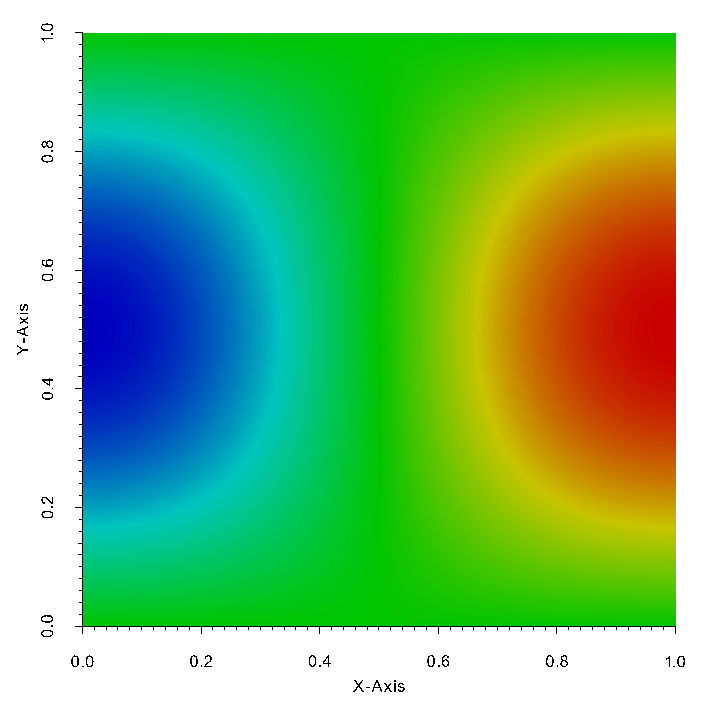
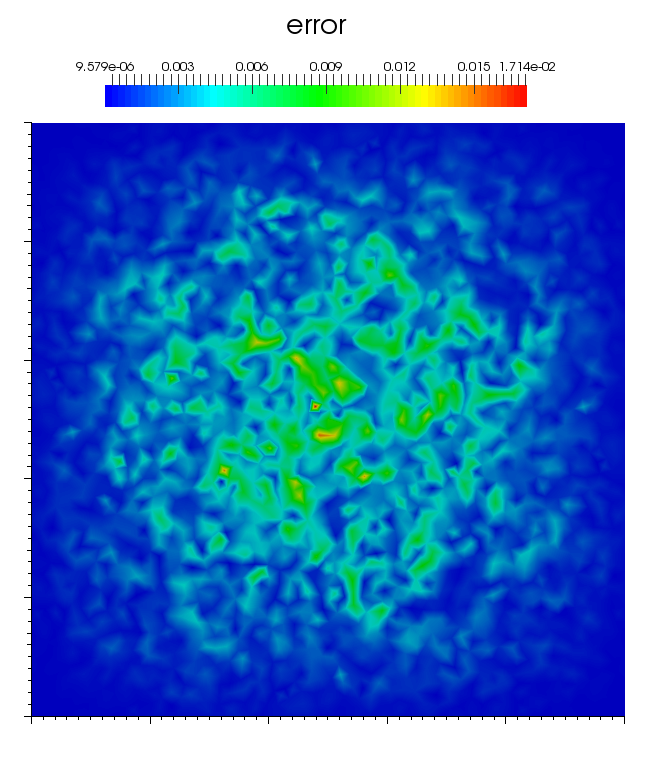
Fig. 6 First component of the solution of the Maxwell 2D problem using Nedelec first family elements, and nodal error

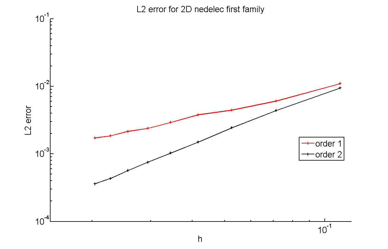
Fig. 7 \(L^2\) errors versus the step \(h\) for 1 and 2 order Nedelec first family approximation