
2D Helmholtz problem coupling FEM and BEM#
We want to solve the acoustic propagation of a plane wave in a heterogeneous medium. In order to do that, we distinguish a domain \(\Omega\) that is heterogeneous, its boundary \(\Gamma\) and the exterior domain \(\Omega_{\mathrm{ext}}\) that is homogeneous:

Fig. 18 Domains for computation: \(\Omega\) the heterogeneous medium, \(\Omega_{\mathrm{ext}}\) the homogeneous exterior domain and \(\Gamma = \partial \Omega\).

Fig. 19 Domains for computation: \(\Omega\) the heterogeneous medium, \(\Omega_{\mathrm{ext}}\) the homogeneous exterior domain and \(\Gamma = \partial \Omega\).
We solve
with \(\eta(x) = 1\) in \(\Omega_{\mathrm{ext}}\), and \(\eta(x)\) that can vary in \(\Omega\), and finally with \(u_i=e^{ikx}\).
We will use: \(\Omega = \left[-0.5, 0.5\right]^2\) and
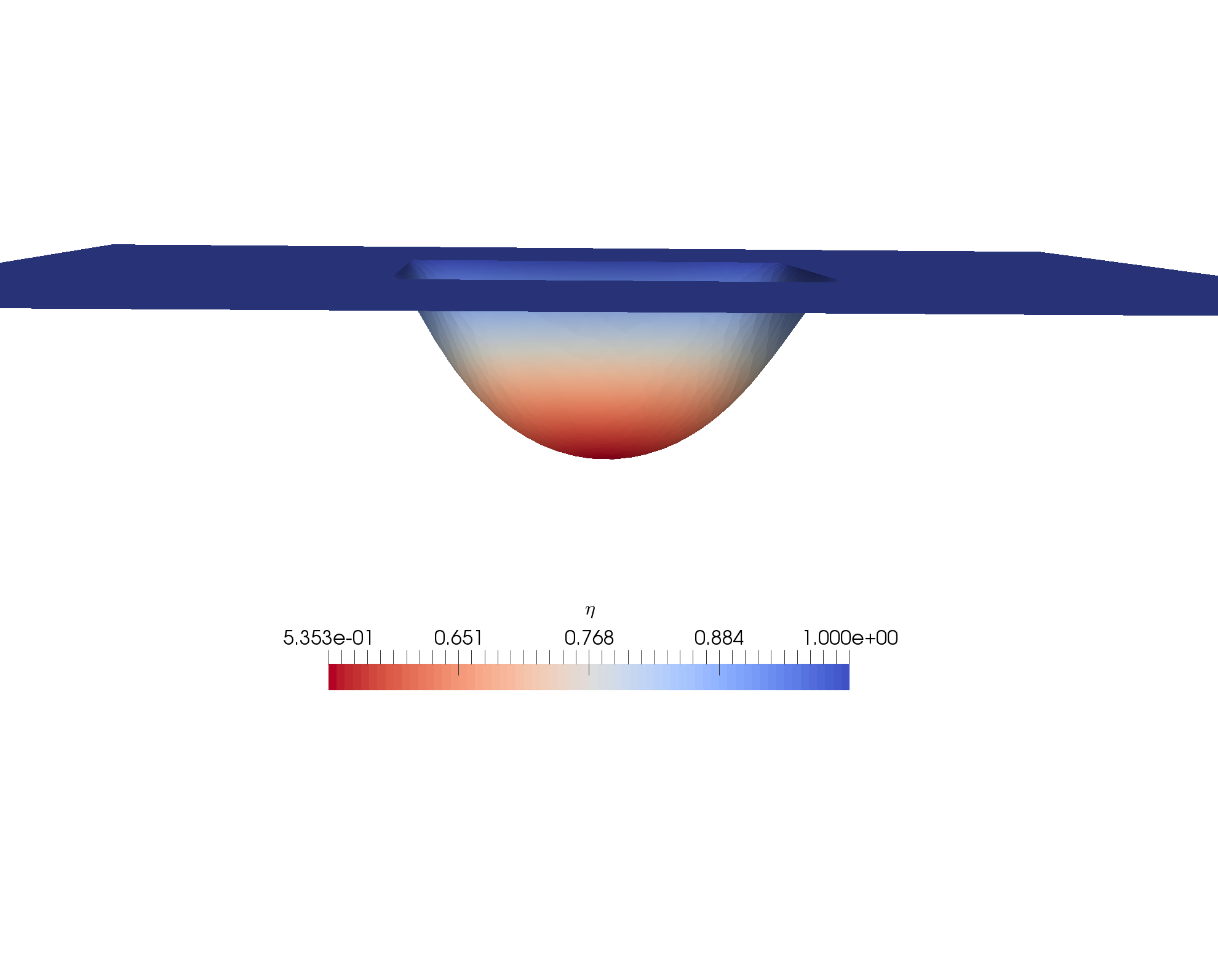
Fig. 20 \(\eta(x)\) in \(\Omega \cup \Omega_{\mathrm{ext}}\)#
We decompose the problem in a coupled system of two equations:
-
in the FEM part, the solution solves the following equation:
\[\Delta u + k^2 \eta^2 u = 0\]which gives the variational formulation
\[\begin{split}\left|\begin{array}{c} \mathrm{Find\;} u \in H^1(\Omega) \mathrm{\;such\;that}: \\ \int_{\Omega} \nabla u(x) \cdot \nabla \bar{v}(x) dx - k^2 \int_{\Omega} \eta^2(x) u(x) \bar{v}(x) dx - \int_{\Gamma} \lambda(x) \bar{v}(x) dx = 0, \quad \forall v \in H^1(\Omega) \\ \end{array} \right.\end{split}\]with \(\lambda = \dfrac{\partial u}{\partial n}\) is the normal trace of \(u\) on \(\Gamma\).
-
in the BEM part, we solve
\[\begin{split}\begin{cases} \Delta u + k^2 u = 0 & \mathrm{\;in\;} \Omega_{\mathrm{ext}} \\ u = -u_i & \mathrm{\;on\;} \Gamma. \end{cases}\end{split}\]The scattered field verifies
\[u_s(x) = - S_{\Gamma}\lambda (x) + K_{\Gamma}u(x), x \in \Omega_{\mathrm{ext}}\]with \(u\) the total field solution of the equation and \(\lambda\) the normal trace of \(u\) on \(\Gamma\), \(S_{\Gamma}\) and \(K_{\Gamma}\) are the single and double layer boundary potentials
\[\begin{split}S_{\Gamma} \phi(x) & = \int_{\Gamma} G(x,y) \phi(y) dy, \notag \\ K_{\Gamma} \phi(x) & = \int_{\Gamma} \dfrac{\partial G(x,y)}{\partial n_y} \phi(y) dy \notag,\end{split}\]and
\[G(x,y) = \dfrac{e^{i k \|x-y\|}}{4 \pi \|x-y\|}.\]Since \(u_s = u - u_i\), and taking the limit when \(x\) goes to \(\Gamma\), we obtain the integral equation
\[\left(\dfrac{I}{2} - K_{\Gamma}\right)u(x) + S_{\Gamma}\lambda(x) = u_i(x), x \in \Gamma.\]The resulting variational formulation for the BEM part is then
\[\begin{split}\left| \begin{array}{c} \mathrm{Find\;} u \in H^{1/2}(\Gamma) \mathrm{\;and\;} \lambda \in H^{-1/2}(\Gamma) \mathrm{\;such\;that}: \\ \dfrac{1}{2} \int_{\Gamma} u(x) \bar{\tau}(x) dx - \int_{\Gamma \times \Gamma} u(y) \dfrac{\partial G(x,y)}{\partial n_y} \bar{\tau}(x) dy dx + \int_{\Gamma \times \Gamma} \lambda(y) G(x,y) \bar{\tau}(x) dy dx \\ \hfill \displaystyle = \int_{\Gamma} u_i(x) \bar{\tau}(x) dx, \forall \tau \in H^{1/2}(\Gamma). \end{array} \right.\end{split}\]
By adding the variational formulations relatives to the two linked problems, we obtain the final variational formulation.
Finally, the solution is obtained directly from \(u\) for the FEM part, and we need to compute the integral representation to obtain \(u_s\), the scattered field, and then to add the incident field to obtain the total field for this problem.
The last step is to merge the FEM solution in \(\Omega\) and the BEM solution in \(\Omega_{\mathrm{ext}}\) to obtain a solution on the whole domain \(\Omega \cup \Omega_{\mathrm{ext}}\) to simplify the visualization.
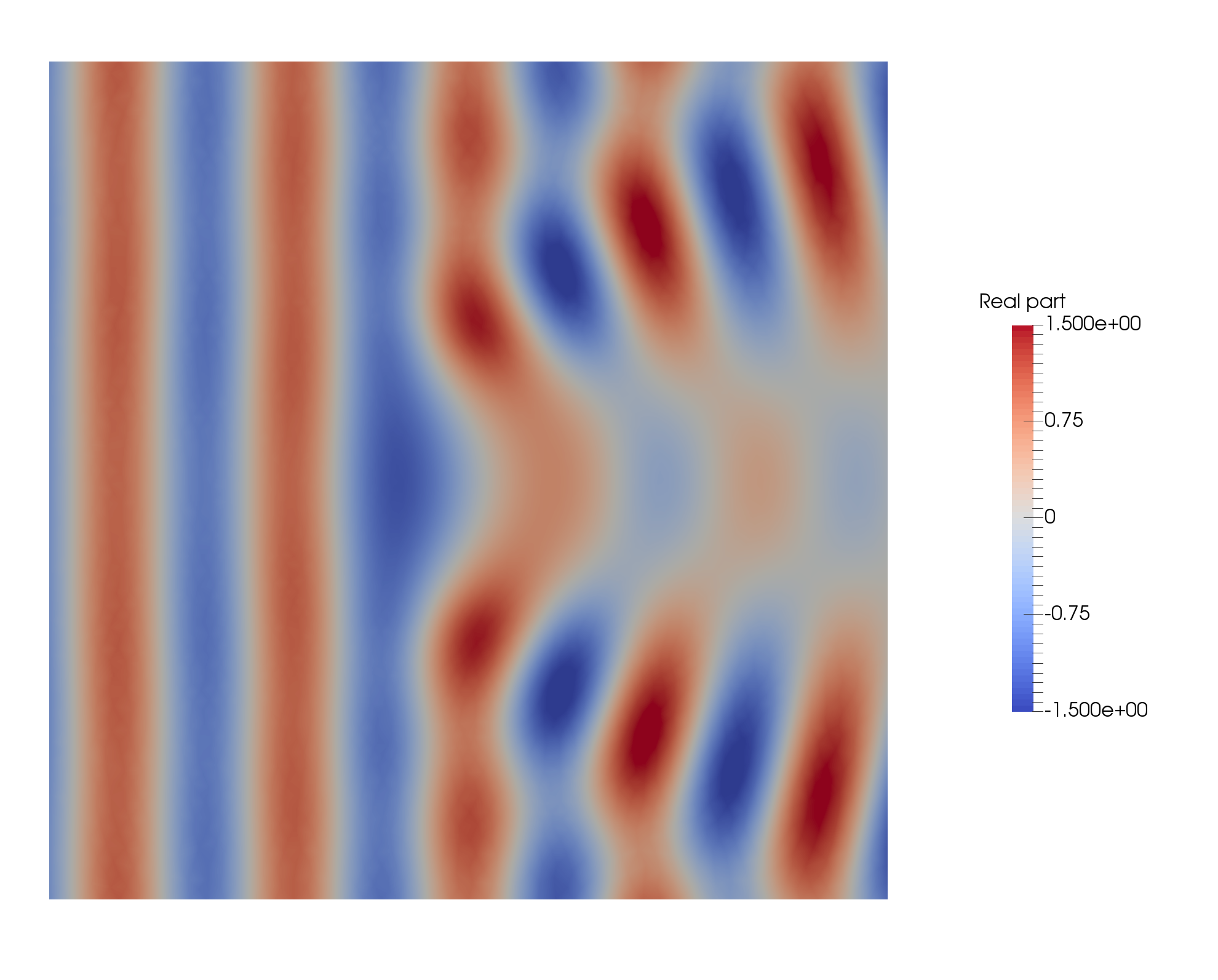
Fig. 21 Solution of the FEM-BEM problem.#
The code of this example follows:
#include "xlife++.h"
using namespace xlifepp;
using namespace std;

// find = eta(x)
Real find(const Point & M, Parameters & pa = defaultParameters)
{
  Real res=1.;
  if (std::max(std::abs(M[0]), std::abs(M[1])) < 0.5)
    res=std::exp(-((M[0]*M[0]-0.25)*(M[1]*M[1]-0.25))/(2.*0.05));
  return res;
}
Real eta2(const Point & M, Parameters & pa = defaultParameters)
{
  Real tmp=find(M);
  return tmp*tmp;
}
Complex g1(const Point& M, Parameters& pa = defaultParameters)
{
  Real k=real(pa("k"));
  Point d(1., 0.);
  return exp(i_*(k*dot(M, d)));
}

int main(int argc, char** argv)
{
  init(argc, argv, _lang=en);   // mandatory initialization of xlifepp
  verboseLevel(10);
  Real k=10.;
  // meshing
  Real hsize=(2*pi_/k)/15.;
  SquareGeo sp(_center=Point(0., 0.), _length=1., _hsteps=hsize, _domain_name="Omega", _side_names="Gamma");
  Mesh m1=Mesh(sp, _shape=triangle, _generator=gmsh);
  Domain omega = m1.domain("Omega");
  Domain gamma = m1.domain("Gamma");
  theCout << "Mesh size = " << hsize << eol;
  theCout << "Number of Triangles = " << m1.nbOfElements() << eol;
  // defining parameter and kernel
  Parameters pars;
  pars << Parameter(k, "k");
  Kernel G=Helmholtz2dKernel(pars);
  Function finc(g1, pars);
  // defining space, unknown and test function
  Space V1(_domain=omega, _interpolation=P1, _name="V1", _notOptimizeNumbering);
  Space V0(_domain=gamma, _interpolation=P1, _name="V0", _notOptimizeNumbering);
  Unknown u1(V1, _name="u1"); TestFunction v1(u1, _name="v1");
  Unknown l0(V0, _name="l0"); TestFunction lt0(l0, _name="lt0");
  theCout << "Nb dofs BEM= " << V0.nbDofs() << " Nb dofs FEM= " << V1.nbDofs() << eol;
  // defining bilinear and linear form
  IntegrationMethods ims(_method=Duffy, _order=15, _bound=0., _quad=defaultQuadrature, _order=12, _bound=1.,
                         _quad=defaultQuadrature, _order=10, _bound=2., _quad=defaultQuadrature, _order=8);
  BilinearForm blf=intg(omega, grad(u1)|grad(v1))-k*k*intg(omega, eta2*u1*v1) - intg(gamma, l0*v1) + 0.5*intg(gamma, u1*lt0)
                  - intg(gamma, gamma, u1*ndotgrad_y(G)*lt0, _method=ims) + intg(gamma, gamma, l0*G*lt0, _method=ims);
  LinearForm lf=intg(gamma, finc*lt0);
  // computing FEM/BEM matrix and right hand side vector
  TermMatrix lhs(blf, _name="lhs");
  TermVector rhs(lf);
  // solving linear system using direct method
  TermVector sol=directSolve(lhs, rhs);

  // Representing the solution FEM and BEM
  SquareGeo Sint(_center=Point(0., 0.), _length=1, _hsteps=hsize, _domain_name="S_int");
  SquareGeo Sext(_center=Point(0., 0.), _length=3, _hsteps=1.5*hsize, _domain_name="S_ext");
  Mesh mrep(Sext+Sint, _shape=triangle, _generator=gmsh);
  Domain S_ext=mrep.domain("S_ext"), S_int=mrep.domain("S_int");
  Domain S=merge(S_ext, S_int, "S");
  Space Vrep(_domain=S, _interpolation=P1, _name="Vrep", _notOptimizeNumbering);
  Unknown ur(Vrep, _name="ur");
  Function Find(find, pars);
  TermVector findex(ur, S, Find);
  saveToFile("findex", findex, _format=vtu); // Representing eta
  TermVector Uint=interpolate(ur, S_int, sol(u1)); // FEM solution (total field)
  saveToFile("Uint", Uint, _format=vtu);

  // Representing of the BEM part
  IntegrationMethods imr(_quad=GaussLegendre, _order=20, _bound=1., _quad=GaussLegendre, _order=10, _bound=2.,
                         _quad=GaussLegendre, _order=5);
  TermVector Uext = - integralRepresentation(ur, S_ext, intg(gamma, G*sol(l0), _method=imr))
                    + integralRepresentation(ur, S_ext, intg(gamma, ndotgrad_y(G)*sol(u1), _method=imr));

  TermVector Uinc(ur, S_ext, finc);
  saveToFile("Uinc", Uinc, _format=vtu); // Incident field
  saveToFile("Uext", Uext, _format=vtu); // scattered field in exterior domain
  TermVector Uext_t = Uext + Uinc;
  saveToFile("Uext_t", Uext_t, _format=vtu); // Total field in exterior domain
  TermVector U=merge(Uint, Uext_t); // Merged FEM and BEM solutions
  saveToFile("U", U, _format=vtu);
  theCout << "Program finished" << eol;
  return 0;
}