Fictitious domain method#

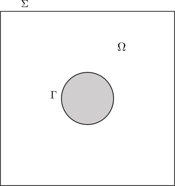
Keywords: PDE:Laplace Method:FEM Method:Mixte FE:Lagrange Solver:Direct

A well-known method to avoid some complex meshes consists in using the fictitious domain method where the boundary condition on an inside obstacle is taken into account by a Lagrange multiplier. To illustrate it, we consider the following 2D Laplace problem in the domain $Ω = C ∖ B (O, R)$ with $C =] 0, 1 [\times] 0, 1 [$ the unit square, $B (O, R)$ the ball with center $C$ and radius $R$ such that $B \subset C$ :

\begin{array}{r} {\begin{cases} - Δ u = f & in Ω \\ u = 0 & on \partial C = Σ \\ u = g & on \partial B = Γ \end{cases} \end{array}

Let us introduce the minimization problem:

min_{\tilde{v} \in \tilde{V} (g)} \frac{1}{2} \int_{C} | \nabla \tilde{V} |^{2} - \int_{C} \tilde{f} \tilde{v}

where

\begin{array}{r} \tilde{V} (g) = {\tilde{v} \in H^{1} (C), {\tilde{v}}_{| Σ} = 0 and {\tilde{v}}_{| Γ} = g} and \tilde{f} = {\begin{cases} f & in Ω \\ 0 & in B \end{cases} . \end{array}

It has a unique solution $\tilde{u} \in \tilde{V} (g)$ such that $\tilde{u} = u$ on $Ω$ and there exists $p \in H^{- \frac{1}{2}} (Γ)$ such that

\begin{array}{r} {\begin{cases} \int_{C} \nabla \tilde{u} . \nabla \tilde{v} - \int_{Γ} p \tilde{v} = \int_{C} \tilde{f} \tilde{v} & \forall \tilde{v} \in H_{0}^{1} (C) \\ \int_{Γ} \tilde{u} q = \int_{Γ} g q & \forall q \in H^{- \frac{1}{2}} (Γ), \end{cases} \end{array}

where the integrals on $Γ$ are to be understood as the duality product on $H^{- \frac{1}{2}} (Γ) \times H^{\frac{1}{2}} (Γ)$ .

The key idea of fictitious domain method is to use two different meshes for $C$ and $Γ$ . As a consequence, the computation of integrals on $Γ$ involves shape functions that lie on two different meshes, inducing interpolation operations from one mesh to the other one. XLiFE++ manages this interpolation operations in a hidden way for the user:

#include "xlife++.h"
using namespace xlifepp;

Real R;

Real f(const Point& P, Parameters& pa = defaultParameters)
{if(norm(P)<=R) return 0.;
 return 2*pi_*pi_*sin(pi_*P(1))*sin(pi_*P(2));}
Real g(const Point& P, Parameters& pa = defaultParameters)
{return sin(pi_*P(1))*sin(pi_*P(2));}

int main(int argc, char** argv)
{
  init(argc, argv, _lang=en); // mandatory initialization of xlifepp
  
  // create meshes (rectangle and circle)
  R=0.2;
  SquareGeo sq(_xmin =0, _xmax = 1, _ymin = 0, _ymax = 1, _hsteps=0.05, _domain_name = "Omega", _side_names="Sigma");
  Disk circle(_center=Point(0.5, 0.5), _radius =R, _hsteps=0.05, _domain_name = "Gamma");
  Mesh meshS(sq, _shape=triangle);
  Mesh meshG(circle, _shape=segment, _generator=gmsh);
  Domain omega  = meshS.domain("Omega"), sigmat = meshS.domain("Sigma"), gammat = meshG.domain("Gamma");
  
  // create spaces and unknowns
  Space Vt(_domain=omega, _interpolation=P1, _name="Vt");
  Unknown ut(Vt, _name="ut"); TestFunction vt(ut, _name="vt");
  Space W(_domain=gammat, _interpolation=P0, _name="W");
  Unknown p(W, _name="p"); TestFunction q(p, _name="q");
  
  // create bilinear forms and Terms
  BilinearForm at = intg(omega, grad(ut)|grad(vt))-intg(gammat, p*vt) - intg(gammat, ut*q);
  BoundaryConditions bcst = (ut|sigmat =0);
  TermMatrix At(at, bcst, _name="At");
  TermVector Ft(intg(omega, f*vt)-intg(gammat, g*q), _name="Ft");
  
  // solve linear system and save the solution to a vtu file
  TermVector Ut = directSolve(At, Ft);
  saveToFile("Ut", Ut, _format=vtu);
  
  return 0;
}

To extract the solution on the real domain $Ω$ , a L2 projection is used:

// create a mesh for Omega
Disk disk(_center=Point(0.5,0.5),_radius =R, _hsteps=0.05, _domain_name = "Obstacle", _side_names="Gamma");
Mesh mesh(rectangle-disk);
Domain omega = mesh.domain("Omega");
Space V(omega,P1,"V"); Unknown u(V,"u"); TestFunction v(u,"v");

//compute L2 projection of ut on omega
TermMatrix M(intg(omega,u*v)), M2(intg(omega,ut*v));
TermVector PUt = directSolve(M,M2*Ut);
saveToFile("PUt",PUt,_vtu);

Note that the computation of the matrix M2 also requires a computation of an integral involving two meshes!

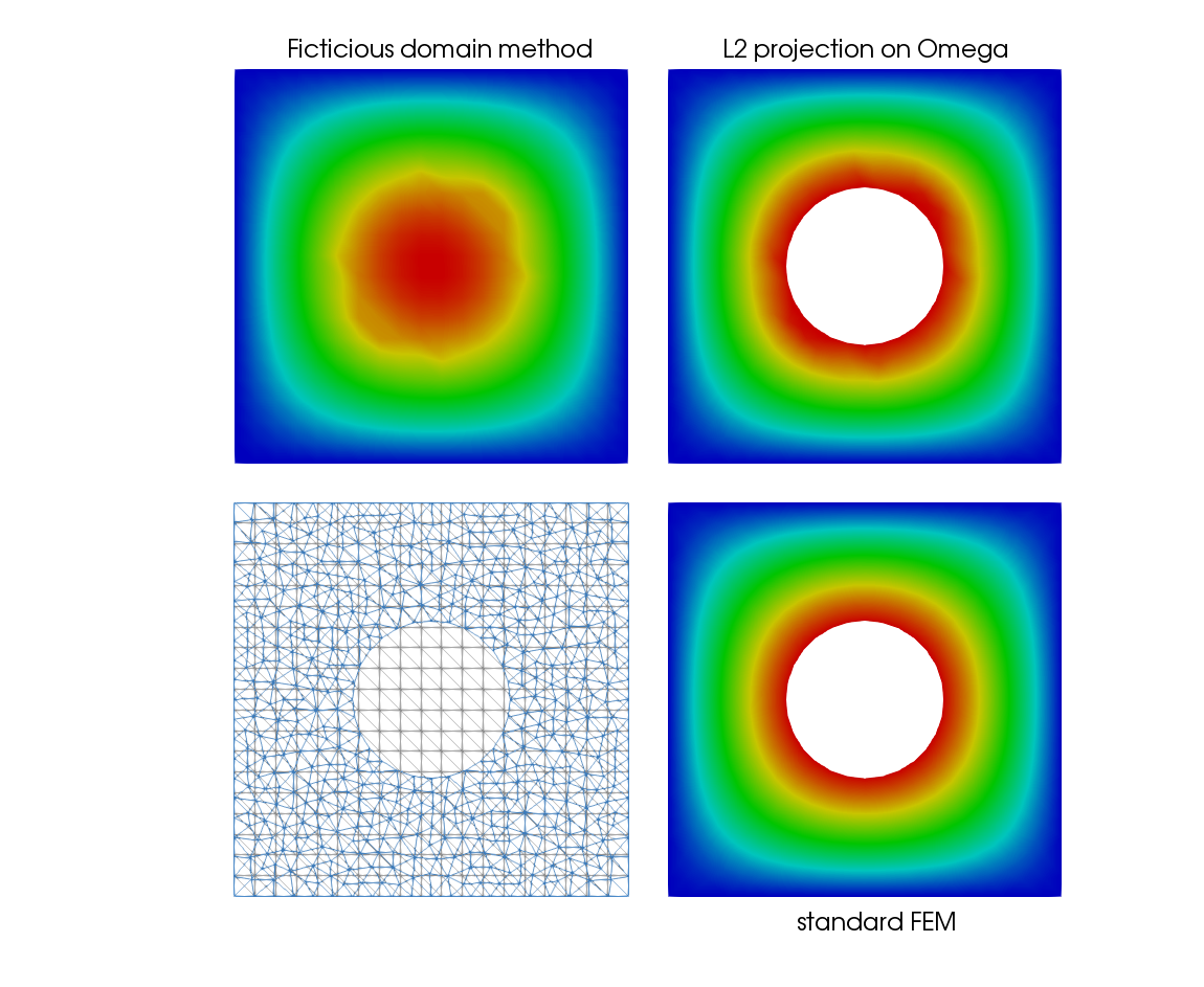
../_images/fictitious_domain.png — Fig. 27 Solution of the Laplace 2D problem with the fictitious domain method#