2D/3D Laplace problem with Neumann condition

Keywords: PDE:Laplace Method:FEM FE:Lagrange Solver:Direct

First, let us consider the case of the homogeneous Neumann condition on \(\partial \Omega\), the boundary of \(\Omega\):

\[\dfrac{\partial u}{\partial n} =0\ \ \ \mathrm{\;on\;} \partial \Omega.\]

The variational formulation we deal with is

\[\begin{split}\left| \begin{array}{c} \mathrm{find\;}u\in V=\left\{v\in L^2(\Omega),\ \nabla v\in (L^2(\Omega))^2\right\} \mathrm{\;such\;that}\\ \displaystyle \int_\Omega \nabla u.\nabla v + a \int_\Omega u\, v =\int_\Omega f\, v \quad \forall v \in V. \end{array} \right.\end{split}\]

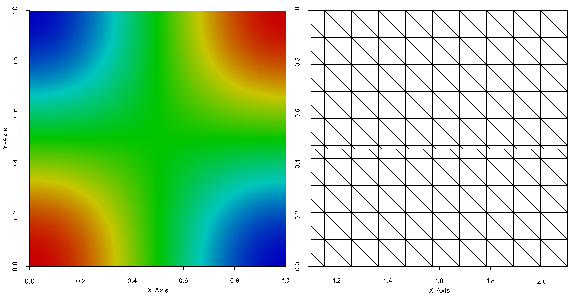
The following main program corresponds to solving this problem on unity square \(\Omega=]0,1[\times ]0,1[\) with \(f(x)=\cos \pi x\cos\pi y\) using P1 Lagrange element (20x20 elements):

#include "xlife++.h"
using namespace xlifepp;

Real cosx2(const Point& P, Parameters& pa = defaultParameters)
{
  Real x=P(1), y=P(2);
  return cos(pi_ * x) * cos(pi_ * y);
}

int main(int argc, char** argv)
{
  init(argc, argv, _lang=en);

  // mesh square
  SquareGeo sq(_origin=Point(0., 0.), _length=1, _nnodes=21);
  Mesh mesh2d(sq, _shape=triangle, _generator=structured);
  Domain omega = mesh2d.domain("Omega");

  // build space and unknown
  Space Vk(_domain=omega, _interpolation=P1, _name="Vk");
  Unknown u(Vk, _name="u");
  TestFunction v(u, _name="v");

  // define variational formulation
  BilinearForm auv = intg(omega, grad(u) | grad(v)) + intg(omega, u * v);
  LinearForm fv=intg(omega, cosx2 * v);

  // compute matrix and right hand side
  TermMatrix A(auv, _name="a(u, v)");
  TermVector B(fv, _name="f(v)");

  // LLt factorize and solve
  TermMatrix LD;
  ldltFactorize(A, LD);
  TermVector U = factSolve(LD, B);

  saveToFile("U_LN", U, _format=vtu);
  return 0;
}

Fig. 25 Solution of the Laplace 2D problem with Neumann condition on the square \([0,1]^2\)

Solving this problem with P2 Lagrange interpolation should be the same except the line defining the space:

Space Vh(_domain=omega, _interpolation=P2, _name="Vh", _optimizeNumbering);

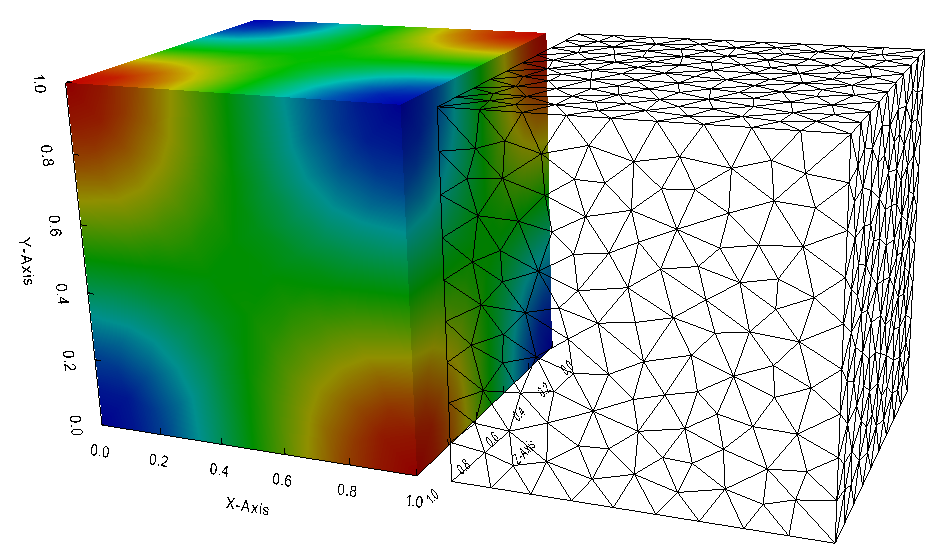
Solving this problem in a 3D domain should be the same except the line defining the mesh and the right-hand side function. For instance, on the unity cube, the mesh construction command using gmsh tool is:

Real f(const Point& P, Parameters& pa = defaultParameters)
{
   Real x=P(1), y=P(2), z=P(3);
   return cos(pi*x) * cos(pi*y) * cos(pi*z);
}
...
Mesh mesh(Cube(_origin=Point(0.,0.,0.), _length=1, _nnodes=10), _generator=gmsh, _name="P1 mesh");
...

Fig. 26 Solution of the Laplace 3D problem with Neumann condition on the unit cube \([0,1]^3\)