1D Laplace problem with Robin condition

Keywords: PDE:Laplace Method:FEM FE:Lagrange Condition:Robin Solver:Direct

The second example shows that XLiFE++ can also handle non-homogeneous Neumann conditions or Robin-Fourier conditions. This problem also involve a Dirichlet condition. Given three real functions \(f_\Omega\), \(\alpha\) and \(f_N\), the problem is:

\[\begin{split}\begin{cases} -u'' + u = f_\Omega & \mathrm{\;in\;} \Omega=\left]a,b\right[ \\ u(a) = 0 & \\ u'(b) + \alpha(b)\, u(b) = f_N(b) & \end{cases}\end{split}\]

Its variational formulation is:

\[\begin{split}\left| \begin{array}{c} \mathrm{Find\;}u\in V=\left\{v\in L^2(\Omega),\ v'\in L^2(\Omega),\ u(a)=0 \right\} \mathrm{\;such\;that}\\ \displaystyle \int_a^bu'(x)\,v'(x)\,dx + \int_a^bu(x)\,v(x)\,dx + \alpha(b)\, u(b) = \int_a^b f(x)\,v(x)\,dx + f_N(b),\ \ \ \forall v\in V. \end{array} \right.\end{split}\]

\(\alpha(b) u(b)\) can be interpreted as \(\displaystyle\int_{\{b\}}\alpha(\gamma) u(\gamma)\,v(\gamma)d\gamma\) and \(f_N(b)\) can be interpreted as \(\displaystyle\int_{\{b\}} f_N(\gamma)\,v(\gamma)d\gamma\) where \(\gamma\) is the variable over the side domain here reduced to a point. This allows to handle these conditions in a uniform syntactic way by defining linear forms as shown in the previous examples.

The following main program corresponds to solving this problem with \(\displaystyle \alpha(x)=\dfrac{7}{2} x^2 - 8x\) using the P10 Lagrange element over the interval \(\displaystyle \left] a, b \right[ = \left] 0,\dfrac{13}{4}\pi\right[\) using 4 elements ; the functions \(f_\Omega(x) = 2\, sin(x)\) and \(f_N(x) = cos(x) + \alpha(x)\, sin(x)\) are chosen so that the solution is \(sin(x)\):

#include "xlife++.h"
using namespace xlifepp;

/*
  Test problem:
    -u" + u = fOm   on the domain Om = [a, b]
      u(a) = 0
      u'(b) + alpha(b) u(b) = fN(b)
*/

Real fctEx (const Point& P, Parameters& pa = defaultParameters)
{ return sin(P[0]); }

Real fctOm (const Point& P, Parameters& pa = defaultParameters)
{ return 2 * sin(P[0]); }

Real alpha (const Point& P, Parameters& pa = defaultParameters)
{ return 3.5*P[0]*P[0] - 8*P[0]; }

Real fctfN (const Point& P, Parameters& pa = defaultParameters)
{ return cos(P[0]) + (3.5*P[0]*P[0] - 8*P[0]) * sin(P[0]); }

int main(int argc, char** argv) {
  init(argc, argv, _lang=en); // mandatory initialization of xlifepp

  // Mesh and domains
  Strings sidenames("x=a", "x=b");
  Segment seg(_xmin=0., _xmax=3.25*pi_, _nnodes=5, _domain_name="Omega", _side_names=sidenames);
  Mesh mesh1d(seg, _generator=structured);
  mesh1d.printInfo();
  Domain Omega = mesh1d.domain("Omega");
  Domain xA = mesh1d.domain("x=a");
  Domain xB = mesh1d.domain("x=b");

  // Space and unknowns
  Space Vh(_domain=Omega, _FE_type=Lagrange, _order=10, _name="Vh");
  Unknown u(Vh, _name="u");
  TestFunction v(u, _name="v");

  // Bilinear forms
  BilinearForm gugv = intg(Omega, grad(u)|grad(v)), uv = intg(Omega, u*v);
  BilinearForm aluv = intg(xB, alpha*u*v);
  LinearForm fOm = intg(Omega, fctOm*v), fN = intg(xB, fctfN*v);

  // Terms with essential conditions
  EssentialConditions ecs = (u|xA = 0);
  TermMatrix A(gugv + uv + aluv, ecs, _name="A");
  TermVector F(fOm + fN, _name="F");

  // Solve linear system and save solution
  TermVector U = directSolve(A, F);
  saveToFile("U", U, _format=matlab);

  // Compare with exact solution
  TermVector Uex(u, Omega, fctEx, _name="Uex");
  theCout << "||U-Uex||inf = " << norminfty(U-Uex) << eol;
  return 0;
}

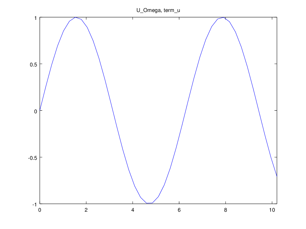
The following figure shows a graphical representation of the solution using Octave (see Solution of the Laplace 1D problem with Dirichlet and Robin conditions):

Fig. 15 Solution of the Laplace 1D problem with Dirichlet and Robin conditions

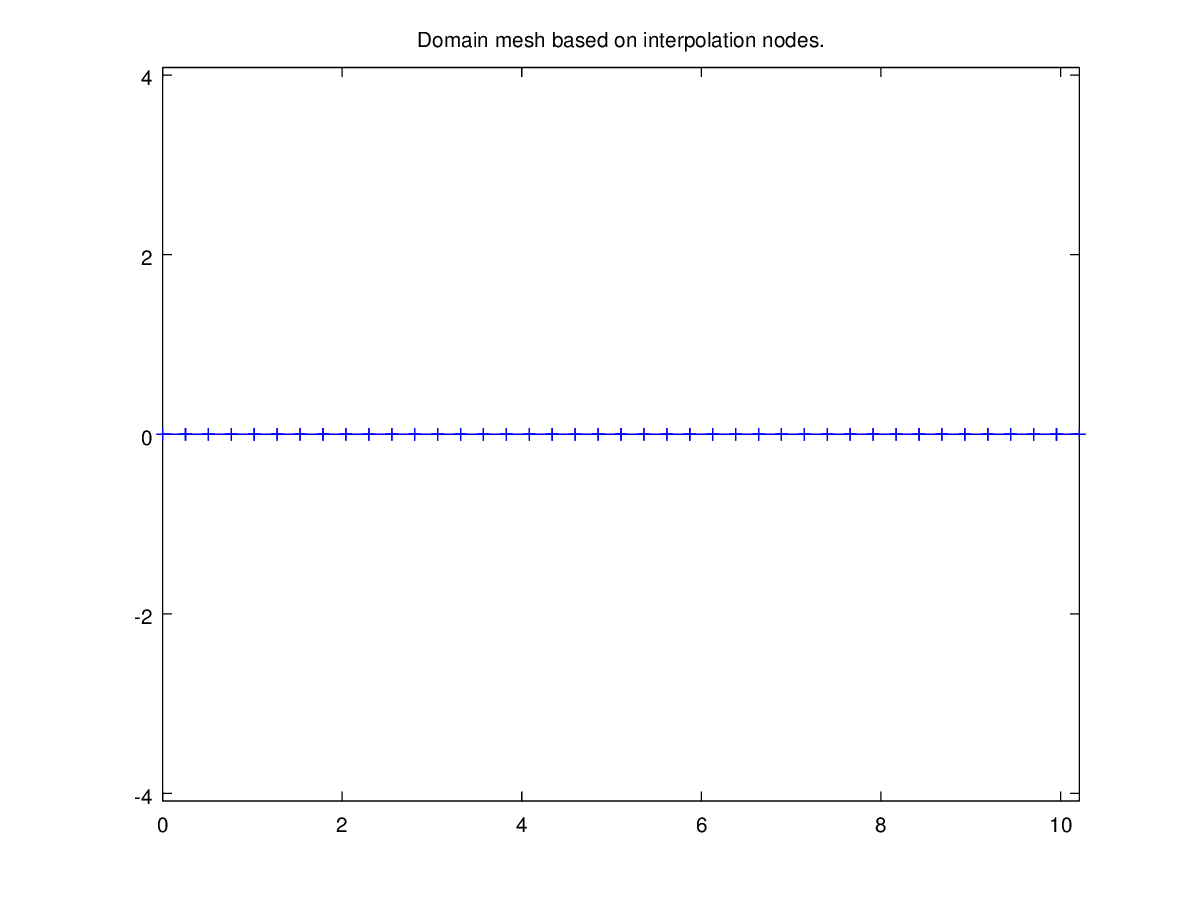
The left figure shows the interpolation nodes which form a uniform distribution of points. This is the default behavior.

Comparing the exact solution \(U_{ex}\) with the computed one \(U\), at the interpolation abscissae, leads to \(||U-U_{ex}||_\infty = 4.44278\times 10^{-10}\), value which is currently printed by the program.

By adding _FE_subtype=GaussLobatto to the Space constructor, one can toggle to the Gauss-Lobatto abscissae which are more suitable with higher interpolation degrees. With this example, choosing these abscissae leads to a better approximation: we then get \(||U-U_{ex}||_\infty = 2.55367\times 10^{-11}\).