Mixed formulation using P0 and Raviart-Thomas elements#

Keywords: PDE:Laplace Method:FEM Method:Coupling Method:Mixte FE:Lagrange FE:RaviartThomas Condition:Dirichlet Solver:Direct

Consider the Laplace problem with homogeneous Dirichlet condition:

\begin{array}{r} {\begin{cases} - Δ u = f & in Ω \\ u = 0 & on \partial Ω \end{cases} \end{array}

Introducing $p = \nabla u$ , it is rewritten as a mixed problem in $(u, p)$ :

\begin{array}{r} {\begin{cases} - div p = f & in Ω \\ p = \nabla u & in Ω \\ u = 0 & on \partial Ω \end{cases} \end{array}

The variational formulation in $V = L^{2} (Ω) \times H (d i v, Ω)$ is to find:

\begin{array}{r} (u, p) \in V ∣ \forall (v, q) \in V, {\begin{cases} - \int_{Ω} div p * v = \int_{Ω} f * v \\ \int_{Ω} u * div q + \int_{Ω} p * q = 0 \end{cases} \end{array}

Note that the Dirichlet boundary condition is a natural condition in this formulation.

The XLiFE++ implementation of this problem using P0 approximation for $L^{2} (Ω)$ and an approximation of $H (d i v, Ω)$ using Raviart-Thomas elements of order 1 is the following:

#include "xlife++.h"
using namespace xlifepp;

Real f(const Point& P, Parameters& pa = defaultParameters)
{ Real x=P(1), y=P(2);
  return 32*(x*(1-x)+y*(1-y));}

int main(int argc, char** argv)
{
  init(argc, argv, _lang=en);
  // mesh square
  SquareGeo sq(_origin=Point(0., 0.), _length=1, _nnodes=21);
  Mesh mesh2d(sq, _shape=triangle, _generator=structured);
  Domain omega=mesh2d.domain("Omega");
  // create approximation P0 and RT1
  Space H(_domain=omega, _interpolation=P0, _name="H", _notOptimizeNumbering);
  Space V(_domain=omega, _FE_type=RaviartThomas, _order=1, _name="V");
  Unknown p(V, _name="p");
  TestFunction q(p, _name="q");  // p=grad(u)
  Unknown u(H, _name="u");
  TestFunction v(u, _name="v");
  // create problem (Poisson problem)
  TermMatrix A(intg(omega, p|q) + intg(omega, u*div(q)) - intg(omega, div(p)*v));
  TermVector b(intg(omega, f*v));
  // solve and save solution
  TermVector X=directSolve(A, b);
  saveToFile("u", X(u), _format=vtu);
  return 0;
}

Using Paraview with the Cell data to point data filter that moves P0 data to P1 data and the Warp by scalar filter that produces elevation, the approximated field $u$ looks like:

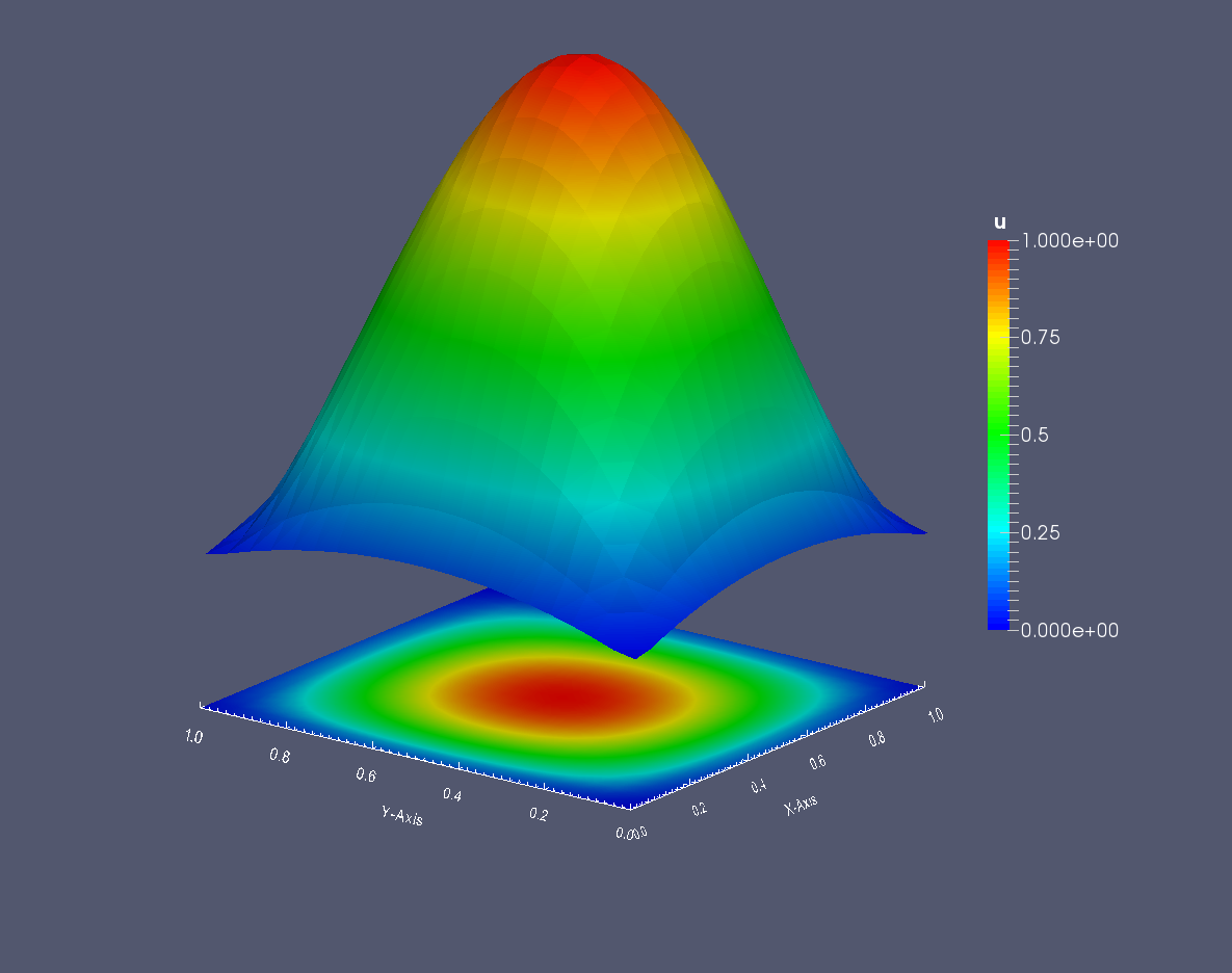
../_images/ex_laplace2d_P0_RT11.png — Fig. 5 Solution of the Laplace 2D problem with mixed formulation P0-RT1 on the unit square $[0, 1]^{2}$ #