Transformations and extrusions#
Transformations on points, geometries and meshes#
XLiFE++ allows you to apply geometrical transformations on Mesh, Geometry and Geometry children objects.
The main type is Transformation. It can be a canonical transformation or a composition of transformations.
Canonical transformations#
In the following, we will consider straight lines and planes. A straight line is fully defined by a point and a direction. The latter is a vector of components (2 or 3). This is a reason why we will write a straight line as follows : \(\left(\Omega, \vec{d}\right)\). A plane is fully defined by a point and a normal vector. This is a reason why we will write a plane as follows : \(\left[\Omega, \vec{n}\right]\).
All canonical transformations are related to classes inheriting from the Transformation class.
Translations#
Point B is the image of point A by a translation of vector \(\vec{u}\) if and only if
A translation can be defined by a vector (size 2 or 3) or by its components:
Reals u;
Real ux, uy, uz;
Translation t1(u), t2(ux, uy), t3(ux, uy, uz);
Important
u can be omitted. If so, its default value is the 3d zero vector. uy and uz can be omitted too. If so, their default value is 0.
2d rotations#
Point B is the image of point A by the 2d rotation of center \(\Omega\) and of angle \(\theta\) if and only if
A 2d rotation is defined by a point and an angle (in radians):
Point omega;
Real angle;
Rotation2d r(omega, angle);
Important
angle can be omitted. If so, its default value is 0 omega can be omitted too. If so, its default value is the 3d zero point.
3d rotations#
Point B is the image of point A by the 3d rotation of axis \(\left(\Omega, \vec{d}\right)\) and of angle \(\theta\) (in radians) if and only if
where \(\displaystyle \vec{n}=\dfrac{\vec{u}}{||\vec{u}||}\) (the unitary direction).
The direction can be defined by an STL vector or by its components:
Point omega;
Vector<Real> d;
Real dx, dy, dz;
Real theta;
Rotation3d r1(omega, d, theta), r2(omega, dx, dy, dz, theta);
Important
In the first syntax, angle can be omitted. If so, its default value is 0. and d can also be omitted. If so, its default value is the 3d zero vector.
In the second syntax, dz can be omitted too. If so, its default value is 0.
Homotheties#
Point B is the image of point A by the homothety of center \(\Omega\) and of factor $k$ if and only if
Point omega(1.,2.,3.);
Real k=2.;
Homothety h(omega, k);
Important
factor can be omitted. If so, its default value is 0. and omega can also be omitted. If so, its default value is the 3d zero vector.
Point reflections#
Point B is the image of point A by the point reflection of center \(\Omega\) if and only if
It is a homothety of factor -1 and same center.
Point omega(1.,2.,3.);
PointReflection h(omega); // omega can still be omitted, as for homothety
2d reflections#
Point B is the image of point A by the 2d reflection of axis \(\left(\Omega,\vec{d}\right)\) if and only if
where \(H\) is the orthogonal projection of \(A\) on \(\left(\Omega,\vec{d}\right)\)
Point omega(1.,2.,3.);
Vector<Real> d(1.,0.,0.);
Real dx=1., dy=0.;
Reflection2d r1(omega, d), r2(omega, dx, dy);
Important
In the first syntax, d can be omitted. If so, its default value is the 2d zero vector and omega can be omitted. If so, its default value is the 2d zero point.
3d reflections#
Point B is the image of point A by the 2d reflection of plane \(\left[\Omega,\vec{n}\right]\) if and only if
where \(H\) is the orthogonal projection of \(A\) on \(\left[\Omega,\vec{n}\right]\).
Point omega(1.,2.,3.);
Vector<Real> n;
Real nx, ny, nz;
Reflection3d r1(omega, n), r2(omega, nx, ny, nz);
Important
In the first syntax, n can be omitted. If so, its default value is the 3d zero vector and omega can be omitted. If so, its default value is the 3d zero point.
Linear transformations#
Any linear transformation can be set from its matrix-vector (\(x\rightarrow \mathbb{A}x+b\)) using the following Transformation constructors:
Transformation(const Matrix<Real>& A, const Vector<Real>& b = Vector<Real>(3,0.))
Transformation(Real a11, Real a12, Real a13, Real a21,Real a22, Real a23,
               Real a31, Real a32, Real a33, Real b1=0, Real b2=0, Real b3=0);
Note
The matrix representation of a transformation can be accessed using the member functions mat and vec. Matrix representations are also available for canonical geometries.
Composition of transformations#
To define a composition of transformations, use the operator * between canonical transformations, an is the following example:
Rotation2d r1(Point(0.,0.), 120.);
Reflection2d r2(Point(1.,-1.), 1.,2.5, -3.);
Translation t1(-1.,4.);
Homothety h (Point(-1.,0.), -3.2);
Transformation t = r1*h*r2*t1;
Composition * has to be understood as usual composition operator \(\circ\) : \(t(P)=r1(h(r2(t1(P))))\).
Note
The matrix representation (mat and vec member functions) is available for composition of transformations.
Applying transformations#
How to apply a transformation ?#
In this paragraph, some transformations are applied to a Cube object, but same functions work for any canonical or composite Geometry. To apply a transformation and modify the input object,
use one of the following functions:
//! apply a geometrical transformation on a Cube
Cube& Cube::transform(const Transformation& t);
//! apply a translation on a Cube
Cube& Cube::translate(std::vector<Real> u = std::vector<Real>(3,0.));
Cube& Cube::translate(Real ux, Real uy = 0., Real uz = 0.);
//! apply a rotation 2d on a Cube
Cube& Cube::rotate2d(const Point& c = Point(0.,0.), Real angle = 0.);
//! apply a rotation 3d on a Cube
Cube& Cube::rotate3d(const Point& c = Point(0.,0.,0.), std::vector<Real> u = std::vector<Real>(3,0.), Real angle = 0.);
Cube& Cube::rotate3d(Real ux, Real uy, Real angle);
Cube& Cube::rotate3d(Real ux, Real uy, Real uz, Real angle);
Cube& Cube::rotate3d(const Point& c, Real ux, Real uy, Real angle);
Cube& Cube::rotate3d(const Point& c, Real ux, Real uy, Real uz, Real angle);
//! apply a homothety on a Cube
Cube& Cube::homothetize(const Point& c = Point(0.,0.,0.), Real factor = 1.);
Cube& Cube::homothetize(Real factor);
//! apply a point reflection on a Cube
Cube& Cube::pointReflect(const Point& c = Point(0.,0.,0.));
//! apply a reflection2d on a Cube
Cube& Cube::reflect2d(const Point& c = Point(0.,0.), std::vector<Real> u = std::vector<Real>(2,0.));
Cube& Cube::reflect2d(const Point& c, Real ux, Real uy = 0.);
//! apply a reflection3d on a Cube
Cube& Cube::reflect3d(const Point& c = Point(0.,0.,0.), std::vector<Real> u = std::vector<Real>(3,0.));
Cube& Cube::reflect3d(const Point& c, Real ux, Real uy, Real uz = 0.);
For instance,
Cube c;
c.translate(0.,0.,1.);
To create a new Cube by applying a transformation on a Cube , use one of the following functions instead:
//! apply a geometrical transformation on a Cube (external)
Cube transform(const Cube& m, const Transformation& t);
//! apply a translation on a Cube (external)
Cube translate(const Cube& m, std::vector<Real> u = std::vector<Real>(3,0.));
Cube translate(const Cube& m, Real ux, Real uy = 0., Real uz = 0.);
//! apply a rotation 2d on a Cube (external)
Cube rotate2d(const Cube& m, const Point& c = Point(0.,0.), Real angle = 0.);
//! apply a rotation 3d on a Cube (external)
Cube rotate3d(const Cube& m, const Point& c = Point(0.,0.,0.), std::vector<Real> u = std::vector<Real>(3,0.), Real angle = 0.);
Cube rotate3d(const Cube& m, Real ux, Real uy, Real angle);
Cube rotate3d(const Cube& m, Real ux, Real uy, Real uz, Real angle);
Cube rotate3d(const Cube& m, const Point& c, Real ux, Real uy, Real angle);
Cube rotate3d(const Cube& m, const Point& c, Real ux, Real uy, Real uz, Real angle);
//! apply a homothety on a Cube (external)
Cube homothetize(const Cube& m, const Point& c = Point(0.,0.,0.), Real factor = 1.);
Cube homothetize(const Cube& m, Real factor);
//! apply a point reflection on a Cube (external)
Cube pointReflect(const Cube& m, const Point& c = Point(0.,0.,0.));
//! apply a reflection2d on a Cube (external)
Cube reflect2d(const Cube& m, const Point& c = Point(0.,0.), std::vector<Real> u = std::vector<Real>(2,0.));
Cube reflect2d(const Cube& m, const Point& c, Real ux, Real uy = 0.);
//! apply a reflection3d on a Cube (external)
Cube reflect3d(const Cube& m, const Point& c = Point(0.,0.,0.), std::vector<Real> u = std::vector<Real>(3,0.));
Cube reflect3d(const Cube& m, const Point& c, Real ux, Real uy, Real uz = 0.);
For instance,
Cube c1;
Cube c2=translate(c1,0.,0.,1.);
Important
A 2d rotation or a 2d reflection cannot be used for geometries defined by 3d points !
What does a transformation really do ?#
Applying a transformation to an object means computing the image of each point defining the object. But it can also change names. When creating a new object using a transformation on a object, names are modified. Indeed, the transformation add a suffix “_prime”. It concerns geometry names and sidenames.
Important
Transforming a Geometry, applies also the transformation on the underlying bounding box.
Geometries extrusions#
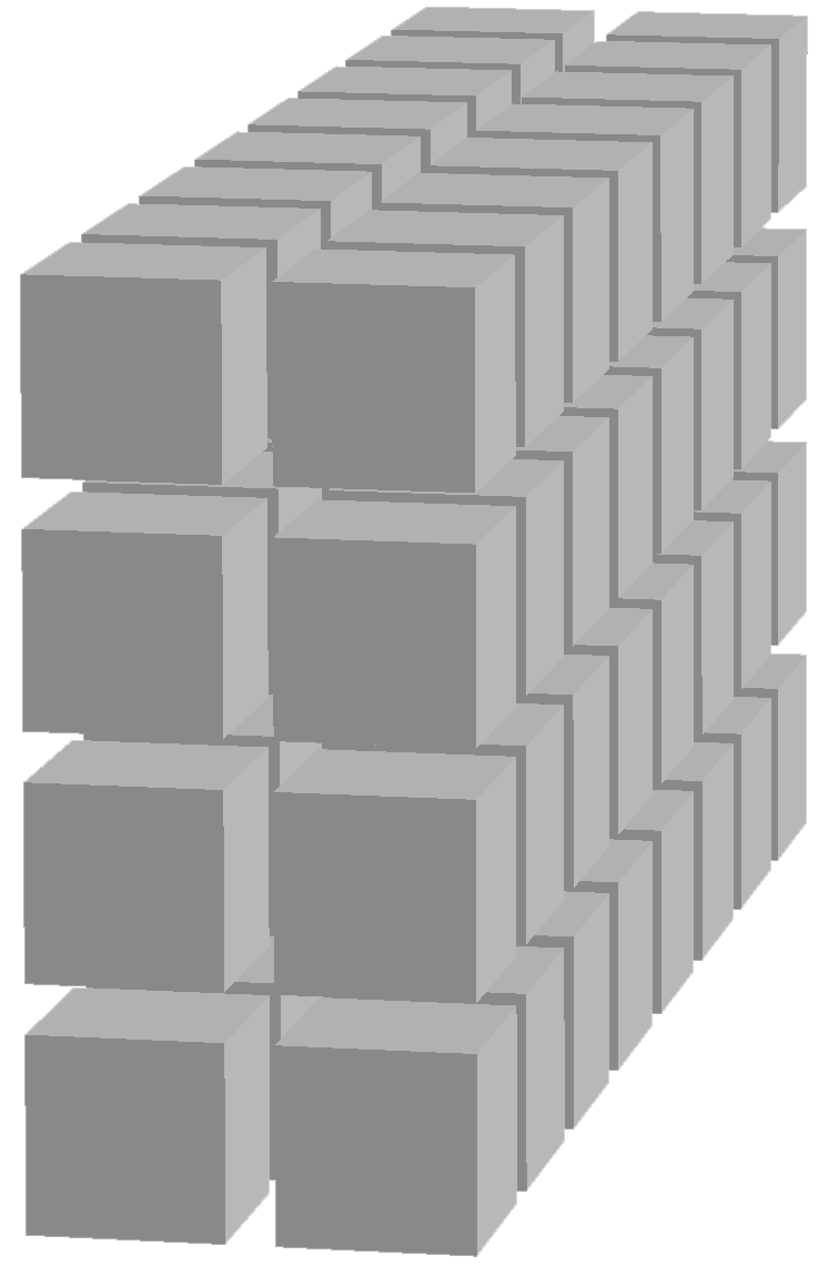
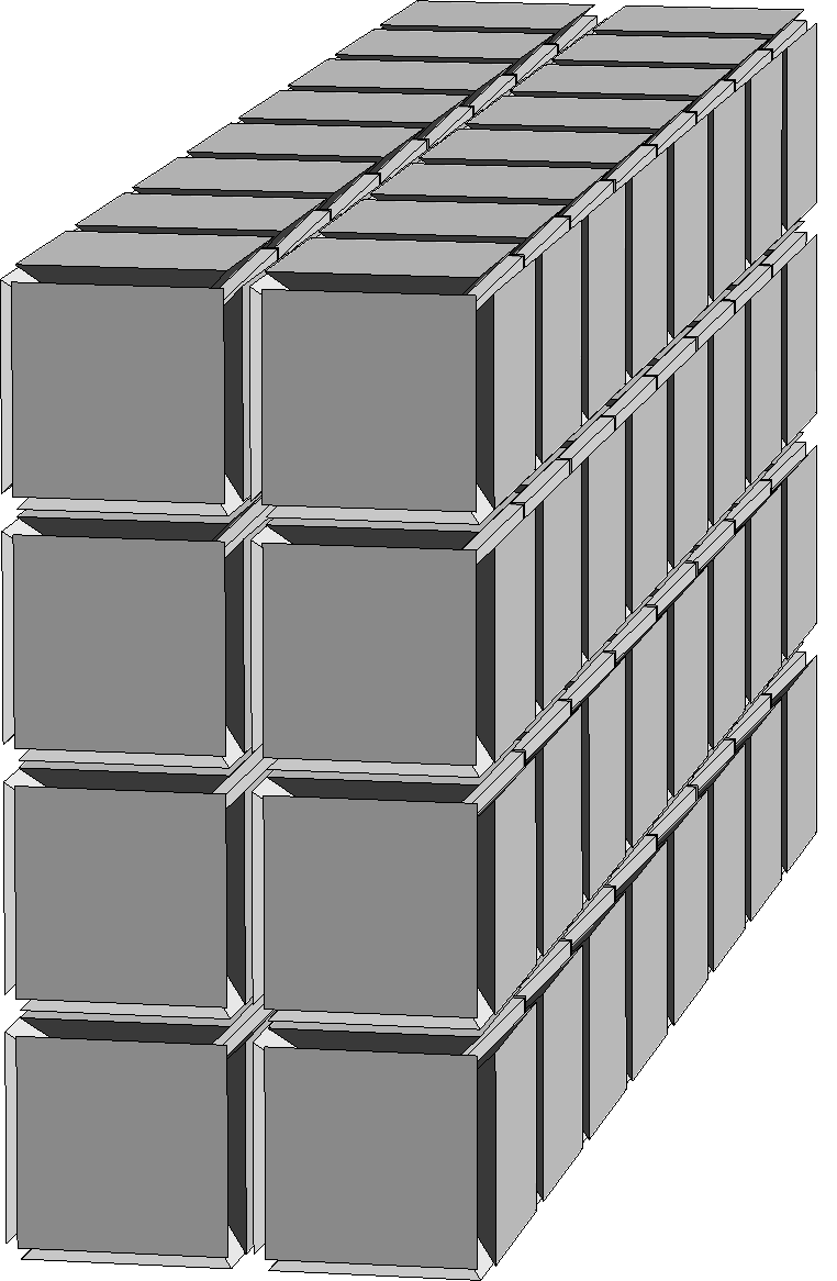
This is another way to define geometries : by extrusion of geometries of lesser dimension. Extruded geometries can be surfaces or volumes, defined by a geometry (the section of the extruded geometry) and a geometrical transformation. This feature can be used to generate meshes with the GMSH interface with some restrictions about the transformation : only translations or rotations are authorized. There is also another parameter : the number of layers. Let’s see the following figures:
On the left, extrusion of a disk by a translation, with 3 layers. On the right, extrusion of a circular arc by rotation, with 4 layers
How to apply an extrusion ?#
XLiFE++ offers 4 variants of the same function to define a Geometry by extrusion, enabling to give the domain name to the extruded geometry and to its sides. Sides numbering is as follows : first, the geometry used as section of the extrusion, second, the other section, and next the lateral surfaces generated by the extrusion.
Geometry extrude(const Geometry& g, const Transformation& t, Number layers);
Geometry extrude(const Geometry& g, const Transformation& t, Number layers, String domName);
Geometry extrude(const Geometry& g, const Transformation& t, Number layers, Strings sidenames);
Geometry extrude(const Geometry& g, const Transformation& t, Number layers, String domName, Strings sidenames);
The Geometry given to the extrude function can be:
-
a canonical one (1D or 2D). Here, a
CircArc:Point b(1.5,-4.,0.); Point c(2.,-3.5,0.); CircArc g(_center=Point(1.5,-3.5,0.), _v1=b, _v2=c, _nnodes=5, _domain_name="BC"); Geometry e2d=extrude(g, Translation(0.,0.,4.), 5, "Omega");
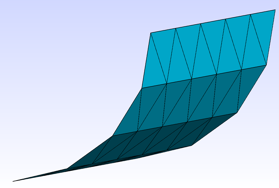
Fig. 102 Extrusion of a circular arc by translation, with 5 layers.#
-
A loop geometry (1D or 2D). Here, a rounded rectangle defines as in Definition of a geometry from its boundary:
Point a(-1.5,-4.,0.); Point b(1.5,-4.,0.); Point c(2.,-3.5,0.); Point d(2.,3.5,0.);
Point e(1.5,4.,0.); Point f(-1.5,4.,0.); Point g(-2.,3.5,0.); Point h(-2.,-3.5,0.);
Segment s1(_v1=a, _v2=b, _nnodes=21, _domain_name="AB");
CircArc c1(_center=Point(3.5,0.5,0.), _v1=b, _v2=c, _nnodes=5, _domain_name="BC");
Segment s2(_v1=c, _v2=d, _nnodes=11,  _domain_name="CD");
CircArc c2(_center=Point(3.5,1.5,0.), _v1=d, _v2=e, _nnodes=5,  _domain_name="DE");
Segment s3(_v1=e, _v2=f, _nnodes=21,  _domain_name="EF");
CircArc c3(_center=Point(0.5,1.5,0.), _v1=f, _v2=g, _nnodes=5,  _domain_name="FG");
Segment s4(_v1=g, _v2=h, _nnodes=11,  _domain_name="GH");
CircArc c4(_center=Point(0.5,0.5,0.), _v1=h, _v2=a, _nnodes=5,  _domain_name="HA");
Geometry g=planeSurfaceFrom(s1+c1+s2+c2+s3+c3+s4+c4,"Omega");
Geometry e3d=extrude(g, Translation(0.,0.,4.), 10, "Omega");
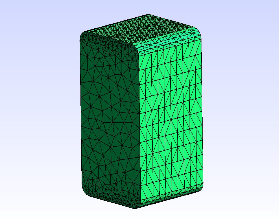
Fig. 103 Extrusion of a rounded rectangle (loop geometry) by a rotation, with 10 layers.#
-
Every composite geometry composed exclusively of a geometry and its holes (1D or 2D). That is to say only operator- or operator-= is used to define the geometry:
Ellipse e1(_center=Point(0.,0.,0.), _v1=Point(4,0.,0.), _v2=Point(0.,5.,0.), _nnodes=12, _domain_name="Omega1", _side_names=Strings("Gamma_1","Gamma_2","Gamma_3","Gamma_4"));
Ellipse e2(_center=Point(1.,2.,0.), _v1=Point(1.5,2.,0.), _v2=Point(1.,3.,0.), _nnodes=12, _domain_name="Omega3", _side_names=Strings("Gamma_9","Gamma_10","Gamma_11","Gamma_12"));
Geometry e3d2=extrude(e1-e2, Rotation3d(Point(5.,0.,0.), 0., 5., 0., pi_/2.), 10, "Omega", "Gamma");
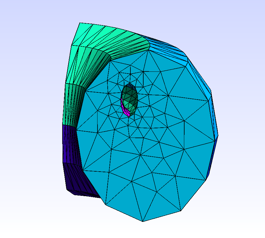
Fig. 104 Extrusion of an ellipse with an elliptical hole by rotation, with 10 layers.#
How to define names of lateral domains of an extrusion ?#
Instead of giving the same name to every lateral surface of an extrusion, it is possible to name each of them, but what about sides numbering ?
First example, let’s take the extrusion of a CircArc :
Point b(1.5,-4.,0.);
Point c(2.,-3.5,0.);
CircArc g(_center=Point(1.5,-3.5,0.), _v1=b1, _v2=c1, _nnodes=5, _domain_name="BC");
Geometry e2d=extrude(g, Translation(0.,0.,4.), 5, "Omega", Strings("Gamma1", "Gamma2");
In Geometries extrusions , point \(b\) is the front below left corner and point \(c\) is the front top right corner. As \(g\) is defined from \(b\) to \(c\), the first lateral side, corresponding to domain \(Gamma1\), will be the edge below. If \(g\) is defined from \(c\) to \(b\), \(Gamma1\) would have corresponded to the edge above.
Second example, let’s take the extrusion of an ellipse with an elliptical hole:
Ellipse e1(_center=Point(0.,0.,0.), _v1=Point(4,0.,0.), _v2=Point(0.,5.,0.), _nnodes=12, _domain_name="Omega1");
Ellipse e2(_center=Point(1.,2.,0.), _v1=Point(1.5,2.,0.), _v2=Point(1.,3.,0.), _nnodes=12, _domain_name="Omega3");
Geometry e3d3=extrude(e1-e2, Rotation3d(Point(5.,0.,0.), 0., 5., 0., pi_/2.), 10, "Omega", Strings("Gamma1", "Gamma2", "Gamma3", "Gamma4", "Gamma5", "Gamma6", "Gamma7", "Gamma8"));
This time lateral surfaces are ordered as follows:
Lateral surfaces from the outer ellipse are ordered the same way as borders of the ellipse
Lateral surfaces from the inner ellipse (and every hole in general) are ordered in the reverse order of borders of the ellipse
Warning
Contrary to _Gmsh, extrusion of a geometry by rotation of angle greater than \(\pi\) is available, by splitting extrusion in 2 half extrusions when angle is not \(2\pi\) or in 4 quarter extrusions when angle is \(2\pi\). As a result, the number of lateral surfaces is multiplicated by 2 or 4.
Example: definition of a conesphere#
To define geometries based on cones, extrusions have to be used. It is the case for the conesphere:
Real rb=1., hc=3.;
Real hs=rb*rb/hc;
Real rs=sqrt(rb*rb + hs*hs);

Point origin(0.,0.,0.), apex(0.,0.,hc), p1(rb,0.,0.), p2(0.,0.,-hs-rs);

Segment s1(_v1=p1, _v2=apex, _hsteps=0.05);
Segment s2(_v1=apex, _v2=origin, _hsteps=0.05);
Segment s3(_v1=origin, _v2=p2, _hsteps=0.05);
CircArc c1(_center=Point(0.,0.,-hs), _v1=p2, _v2=p1, _hsteps=0.05);
Disk d1(_center=0.5*p1, _v1=0.5*p1+Point(0.2*rb,0.,0.), _v2=0.5*p1+Point(0.,0.,0.2*rb), _domain_name="Sigma", _hsteps=0.05);

Geometry base=planeSurfaceFrom(s2+s3+c1+s1, "Gamma");
Geometry g=extrude(base, Rotation3d(Point(0.,0.,0.), 0., 0., 1., 2.*pi_), "Omega1", Strings("Gamma1", "Gamma2", "Gamma3", "Gamma4", "Gamma5", "Gamma6", "Gamma7", "Gamma8"));
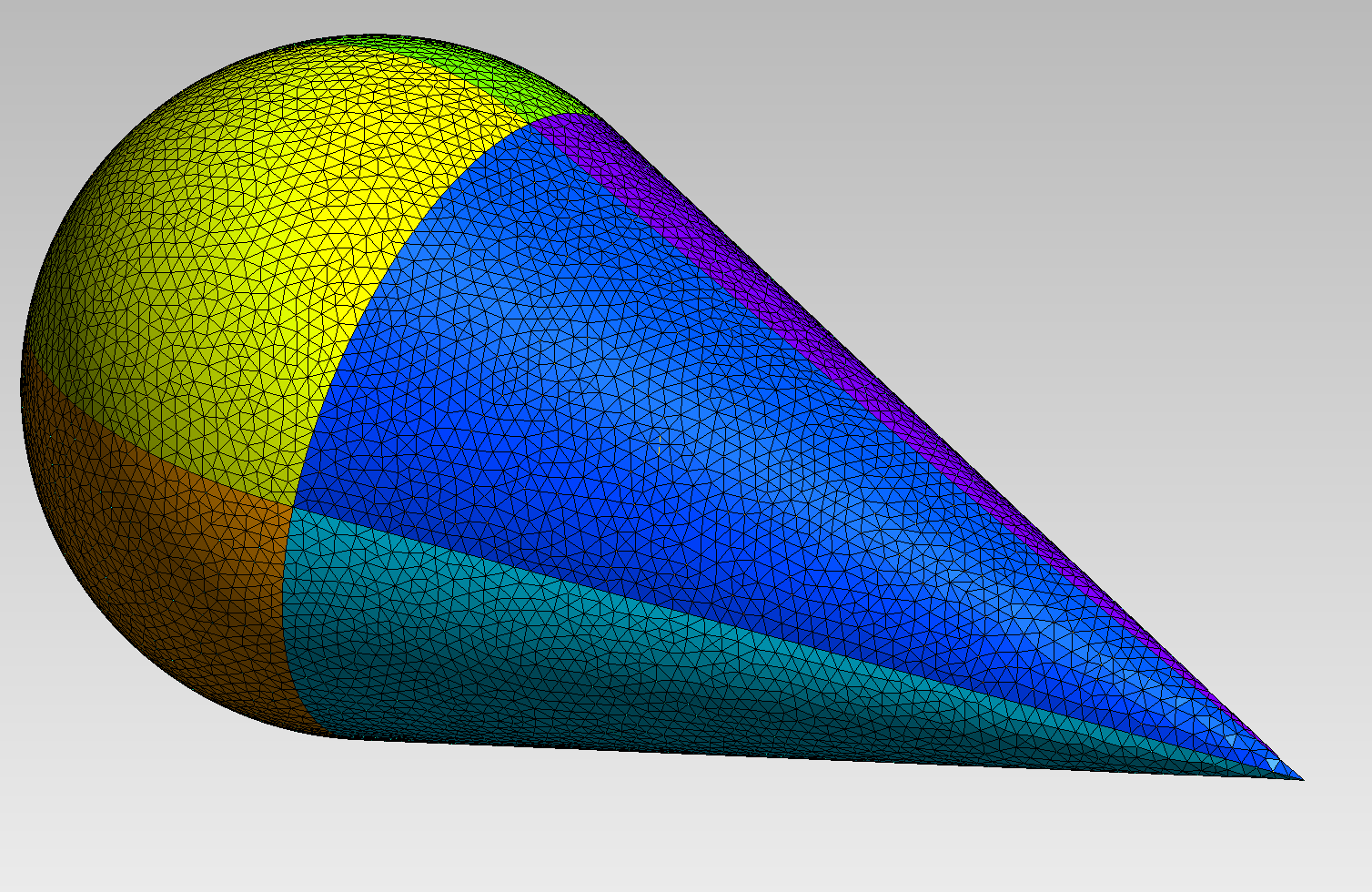
Fig. 105 Mesh of a conesphere.#
Mesh transformations#
Transformations on meshes#
Geometrical transformations on meshes work as on geometries. Please see Transformations on points, geometries and meshes for definition and use of transformations routines.
Then, if you want to apply a transformation and modify the input object, you can use one of the following functions:
translate to apply a translation
rotate2d to apply a rotation 2d
rotate3d to apply a rotation 3d
homothetize to apply a homothety
pointReflect to apply a point reflection
reflect2d to apply a reflection 2d
reflect3d to apply a reflection 3d
For instance:
Mesh m(...);
m.translate(0.,0.,1.);
However, if you want now to create a new Mesh by applying a transformation on a Mesh, you should use one of the related external functions instead.
For instance:
Mesh m(...);
Mesh m2=translate(m, 0.,0.,1.);
Mesh extrusion#
Instead of extruding a geometry, it is possible to extrude a 1D or 2D mesh (section) by applying a geometric transformation to it. To do this, use the function extrude.
Mesh extrude(s_mesh, tranformation, [[key-value1,[key-value2]], ...])
where
-
the mesh of the section (
s_mesh) may be eithera 1d mesh made of segments, the extruded mesh is then a 2d mesh made of quadrangles
a 2d mesh made of triangles or quadrangles, the extruded mesh is then a 3d mesh made of prisms or hexahedra.
-
the transformation may be either
a
Transformationobject handling a tranlsation, a rotation or a combination of basic transformations; the same transformation being applied to each section of the extrusiona collection of
Transformationobjects, each transformation being applied to one section of the extrusion. The number of transformations has to be equal to the number of layers of the extrusion.-
a c++ function describing the extrusion path, with the following form:
Vector<real_t> path(const Point&, Parameters&, DiffOpType);
Key values (up to 5) can be specified to control the extrusion process:
_layersto give the number of layers (mandatory)_centerto give the center of rotation when using a curve parameterization (computed by default as the barycenter of the input section)_init_transformationto specify a tranformation to apply to the reference section before extruding it (none by default)_naming_domainto control the naming of domains (noName,globalName,indexedName)_naming_sectionto control the naming of sections(noName,globalName,indexedName)_naming_sideto control the naming of boundaries (noName,globalName,indexedName)
The meaning of the naming arguments is
noName: no domains, no section domains, noboundaries domains are created. The full domain is always created and named “#Omega”.globalName: only some global extruded domains, a domain including end sections or some global boundary domains included all boundary domains are created (domain names are postfixed _e).indexedName: for each layer, one extruded domain, section domain or boundary domains are created (domain names are postfixed _0, _1,… or _e0, _e1, …).
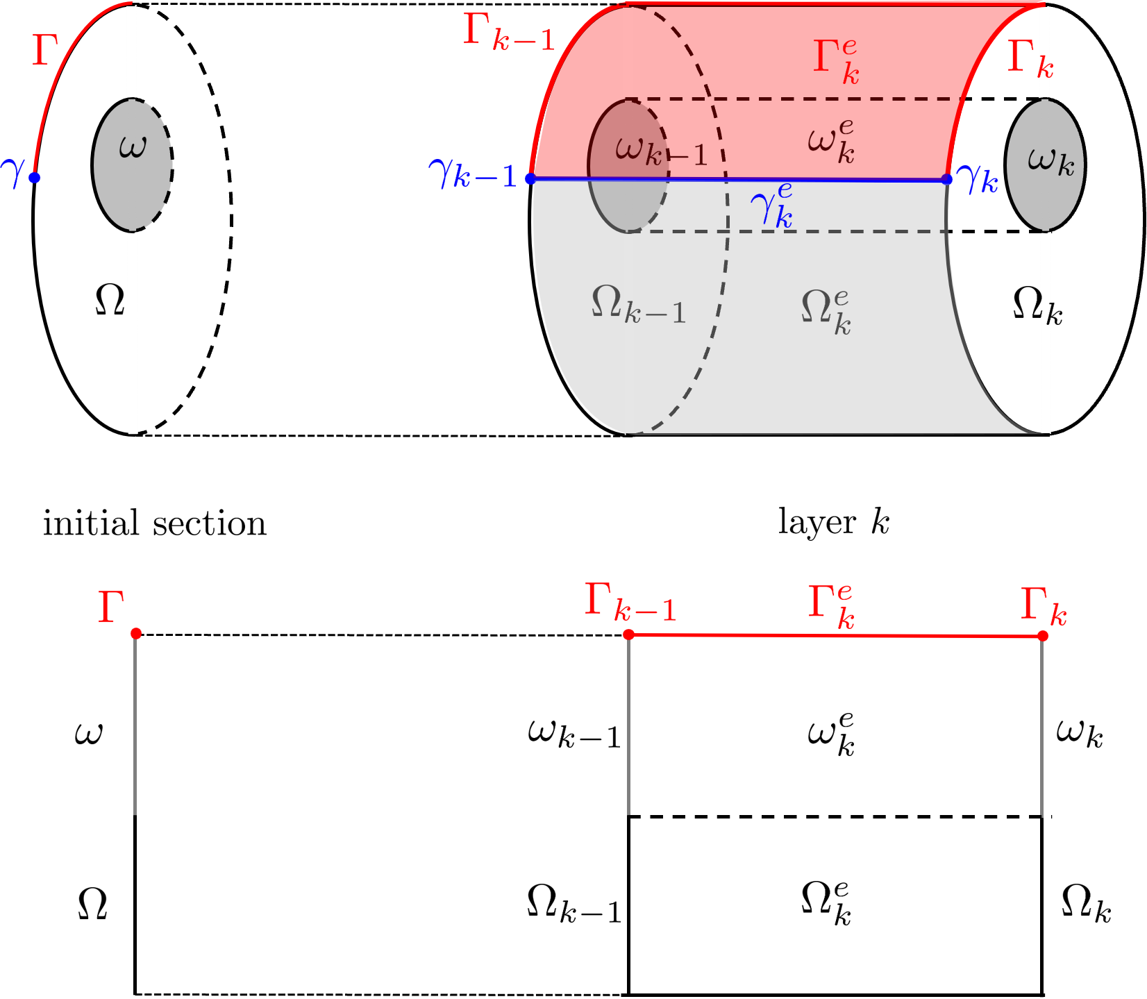

The following figure illustrates the naming rules of domains when meshing a tubular domain using crown mesh extrusion:
Disk dext(_center=Point(0.,0.), _radius=1., _nnodes=20, _domain_name="Omega", _side_names="Sigma");
Disk dint(_center=Point(0.,0.), _radius=0.5, _nnodes=10, _side_names="Gamma");
Mesh crown(dext-dint, _generator=gmsh);
Mesh tube(crown, Translation(0,0,.1), _layers=10, _naming_domain=1, _naming_section=1, _naming_side=1);
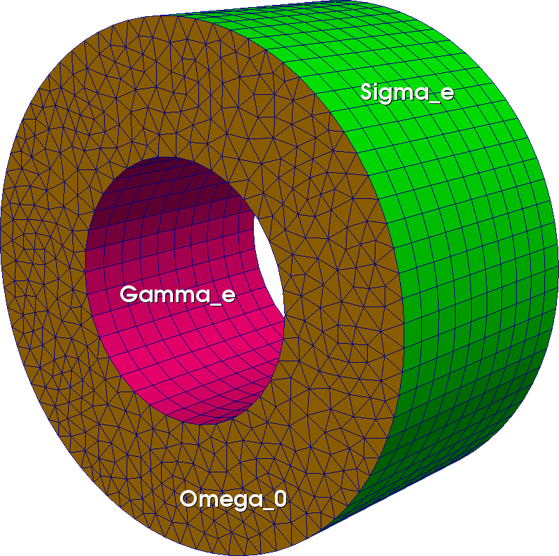
Fig. 106 Tube prismatic mesh from extrusion of a crown mesh#
Example 1: extrusion of a disk using a rotation leading to a torus
Here a 3d rotation of angle \(\frac{\pi}{20}\) is applied to each section and _layers key-value specifies the number of layers (40). Note that in that case, a full turn is done and the last section coincides with the first section, the nodes being not duplicated.
..code:
Mesh mdi(Disk(_center=Point(0.,0.), _radius=1., _nnodes=8), _shape=_triangle);
Mesh m=extrude(mdi, Rotation3d(_center=Point(3.,0.,0.), _axis={0.,1.,0.}, _angle=2*pi_/40), _layers=40);
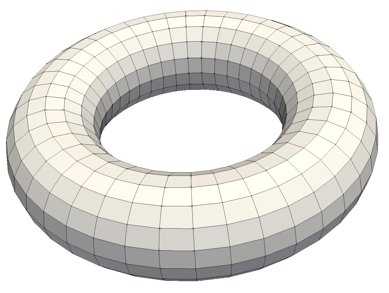
Fig. 107 Extrusion using a rotation leading to a torus#
Example 2: extrusion of a rectangle using a combination of transformations
The transformation may be a combination of transformations (see Transformations on points, geometries and meshes for more details):
Mesh mr(Rectangle(_xmin=0, _xmax=1, _ymin=1, _ymax=3, _nnodes=Numbers(6, 10)), _shape=_triangle, _order=1, _generator=_structured);
Mesh m=extrude(mr, Translation(0.,0.1,0.)*Rotation3d(Point(3.,0.,0.), Reals(0.,1.,0.), 2.5*pi_/100), _layers=100);
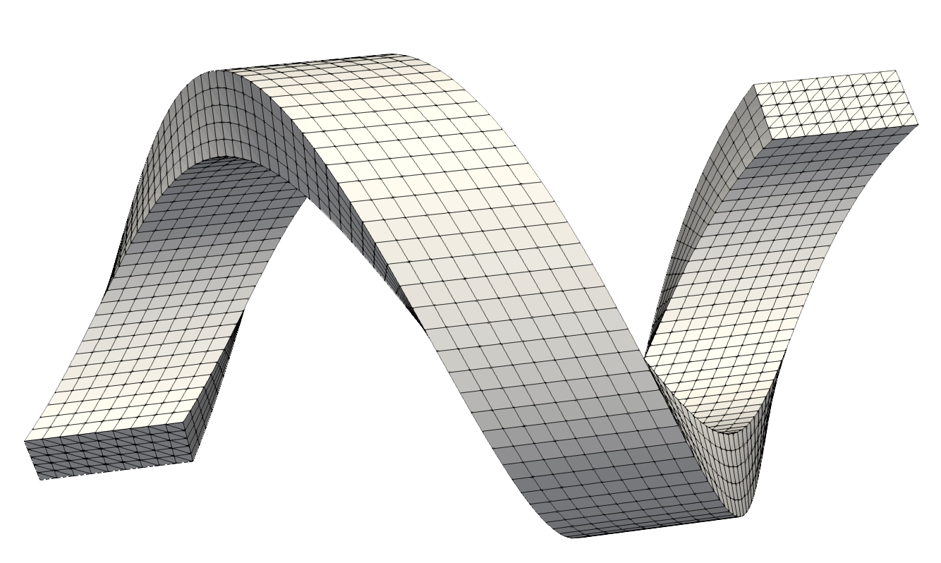
Fig. 108 Extrusion using a combination of transformations#
Example 3 : extrusion of a rectangle using a list of transformations
Instead of specifiying a transformation, it is possible to specify the list of transformations to apply to the sections:
Mesh mr(Rectangle(_xmin=0, _xmax=1, _ymin=1, _ymax=3, _nnodes=Numbers(6, 10)), _shape=_triangle, _order=1, _generator=_structured);
Translation tran(0.2,0.,0.);
Rotation3d rot1(Point(3.,0.,0.),Reals(0.,1.,0.),pi_/40);
Rotation3d rot2(Point(5.,0.,6.),Reals(0.,1.,0.),-pi_/40);
std::vector<Transformation*> trs(50);
for (number_t i=0; i<20; i++)  { trs[i]=&rot1; trs[i+30]=&rot2; }
for (number_t i=0; i<10; i++)  { trs[i+20]=&tran; }
Mesh m=extrude(mesh2dP1, trs, _naming_domain=1);
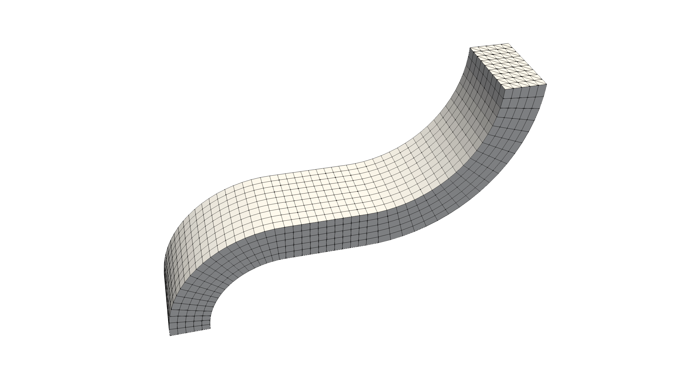
Fig. 109 Extrusion using a list of Transformations#
Example 4 : extrusion of a disk using a path parametrization
To deal with more general extrusions, a C++ function giving the parametrization of the extrusion path: \(t\in[0,1]\rightarrow \gamma(t)\in \mathbb R^d\) can be given. Be cautious, the parametrization has to statisfy \(\gamma(0)=0\) and \(\gamma'(0)=n_s\) where \(n_s\) is the normal vector to the section to be extruded. The extrusion works as following:
the nodes \(M_0\) of section \(S_0\) are translated: \(M_k=M_0+\gamma(\frac{k}{n})\)
then, a rotation defined from the center \(C_k=C_0+\gamma(\frac{k}{n})\) and the two vectors \(n_0,\ \gamma'(\frac{k}{n})\) is applied to the nodes \(M_k\)
By default, the rotation center \(C_0\) is the barycenter of all nodes of the section \(S_0\) but it can be changed using the key-value _center. Note that this process guarantees that all sections are orthogonal to the extrusion curve.
Reals gamma(const Point& P, Parameters& par, DiffOpType dop)
{
  real_t t=P(1);
  if (dop==_dt) return Reals{16*pi_*std::sin(4*pi_*t), 0., 40.};
  return Reals{2*(1-std::cos(4*pi_*t)), 0., 40*t};6
}

Mesh mdi(Disk(_center=Point(0.,0.), _radius=1., _nnodes=8), _shape=_triangle, _generator=subdiv);
Mesh m=extrude(mdi, gamma, _layers=100);
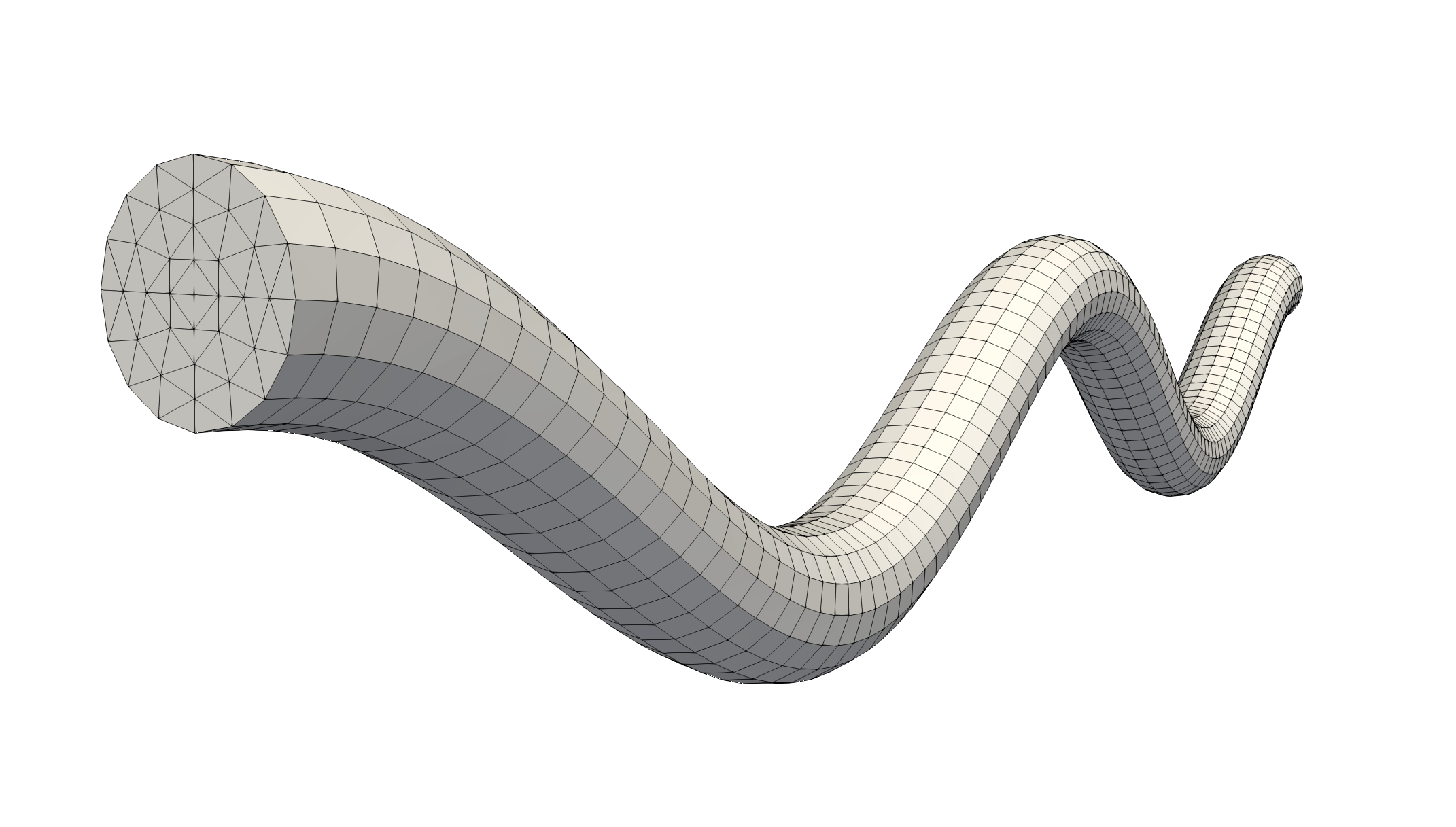
Fig. 110 Extrusion using a curve parametrization#
Tip
The orientation of normal vector to the section to be extruded is not predictable. But using the routine setNormalOrientation it can be set:
Mesh mdi(Disk(_center=Point(0.,0.), _radius=1., _nnodes=8), _shape=_triangle);
mdi.domain(0).setNormalOrientation(_towardsInfinite,Point(0.,0.,-1.));
where the given point (here (0.,0.,-1.)) specifies an ‘interior’ point.
Danger
If curvature radius is too small compared to the section size, the extrusion process may lead to incoherent domain!
Mesh refinement#
It is possible to refine an existing mesh of order 1: a new mesh is created using the subdivision generator mentioned above. It is a uniform refinement, say, all the elements are subdivided in a same way. The corresponding constructor is defined as follows:
Disk d(_center=Point(0.,0.), _radius=1., _nnodes=5);
Mesh md(d, _generator=gmsh, _shape=triangle);
Mesh md1(md, _refinement_depth=1);
Mesh md2(md, _refinement_depth=2);
This builds the meshes md2 and md2 which are obtained by subdividing, respectively, once and twice the mesh md:

Fig. 111 Refine once and twice the P1 mesh of a disk.#
The optional keys are:
_refinement_depth: the refinement depth of the subdivision generator. 0 means no refinement (the default value).
_order: by using it, it possible to increase the order of the refined mesh (defaut value is 1).
Note
Up to now, there is no adaptative refinement tool!
Splitting mesh element#
Sometimes it may be useful to split elements into elements of another type, for instance to produce mesh of pyramids that are not provided by standard meshing software products. To do this, the routine split is available:
Cuboid c(_xmin=0, _xmax=1, _ymin=1, _ymax=3, _zmin=1, _zmax=5, _nnodes={3, 5, 9});
Mesh meshQ1(c, _shape=hexahedron, _generator=structured, _name="Q1 mesh");
Mesh meshPyramid=split(meshQ1, pyramid, "Py1 mesh");
Fig. 112 Hexahedron mesh split to pyramid mesh.#
Note
Up to now, only one splitting process is available: hexahedron of order 1 into six pyramids of order 1, based on the hexahedron faces and the centroid of the hexahedron as tip.
Merging meshes#
It is possible to merge some meshes of same dimension. They can share common parts or common boundaries but with same elements/nodes. If elements or nodes on common parts do not coincide, the resulting mesh would not be conform to do finite element approximations. The merging process combines the elements and nodes of the meshes, eliminating duplicate elements or duplicate nodes. Domains with same name are also merged, names being preserved. The new whole domain is created with default name #Omega or one given and shared boundary domains are merged on demand (default).
Mesh m1(...);
Mesh m2(...);
Mesh m3(...);
m1.merge(m2,[mergeSharedBoundary=true],[name="#Omega"]);//merging m2 with m1
m1.merge(m3,[mergeSharedBoundary=true],[name="#Omega"]);//merging m2, m3 with m1
Mesh m = merge(m1,m2,m3,[mergeSharedBoundary = true],[name = "#Omega"]);
// alternate syntax merging m1,m2 and m3 in a new mesh m (up to 5 meshes)
As an example:
Rectangle R1(_xmin=0, _xmax=1, _ymin=1, _ymax=3, _nnodes={6,10});
Rectangle R2(_xmin=1, _xmax=2, _ymin=1, _ymax=3, _nnodes={3, 5});
Mesh mP1(R1, _shape=triangle, _generator=structured, _name="P1 mesh");
Mesh mQ1(R2, _shape=quadrangle, _generator=structured, _name="Q1 mesh");
Mesh mP1Q1 = merge(mP1,mQ1);

Rectangle R3(_xmin=1, _xmax=2, _ymin=1, _ymax=3, _nnodes={6,10});
Mesh mQ1a(R3, _shape=quadrangle, _generator=structured, _name="Q1 mesh a");
mP1Q1 = merge(mP1,mQ1a);
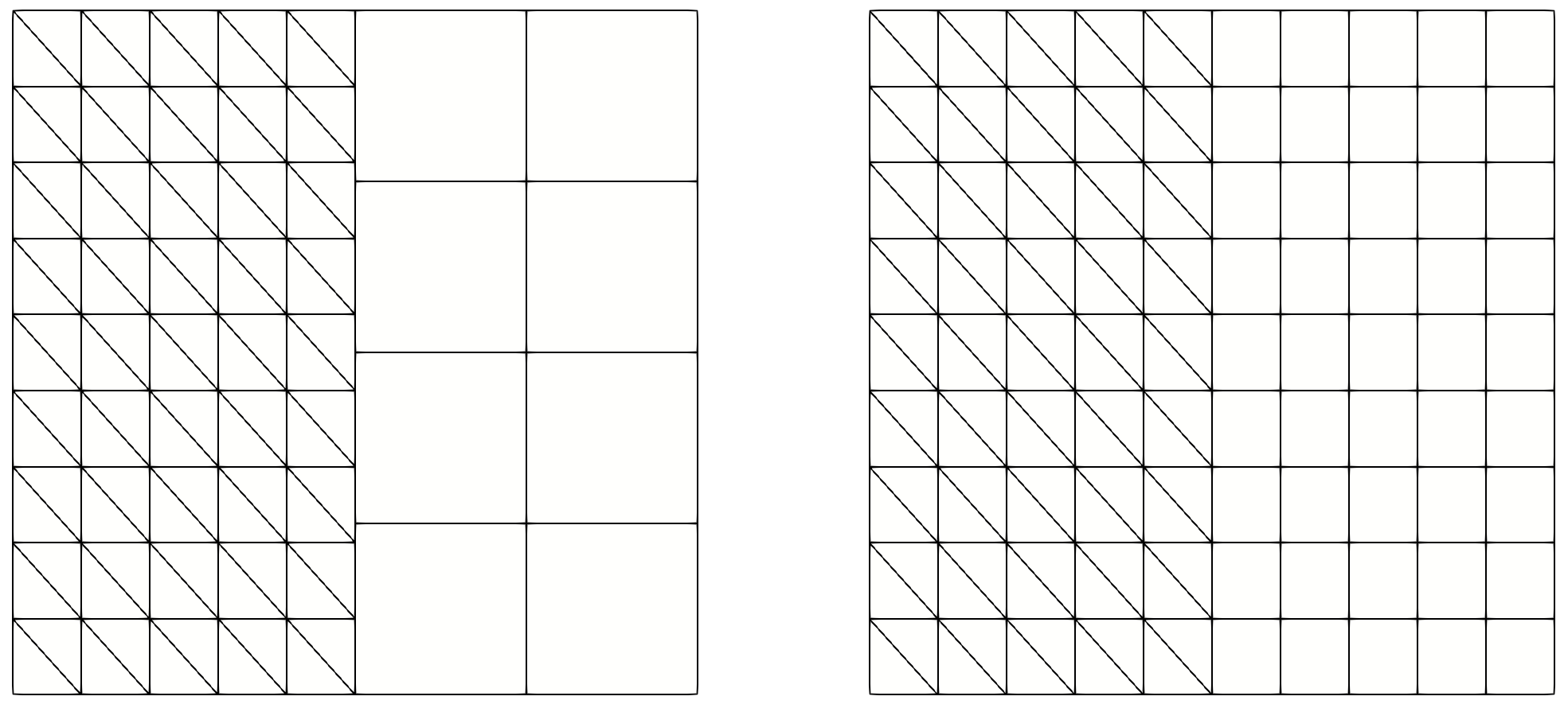
Fig. 113 Non-conforming and conforming merging of a triangular mesh with a quadrangular mesh.#
In the merging process the following rules are applied:
all named domains of original meshes are preserved, with the same names,
if two different domains have the same name, they are merged,
-
if two side domains define an interface (same nodes) in the merging process and do not have the same name, say domname1 and domname2:
if
mergeSharedBoundaryis true, a new domain named domname1_domname2 is created and the original ones are deletedif
mergeSharedBoundaryis false, the original domains domname1 and domname2 are retained
if two side domains define an interface in the merging process and have the same name, say domname, only one domain remains, again named domname and regarded as an interface.
Attention
If two side domains with the same name have a common part which is not the whole side domain, the merging process fails and an error is raised.
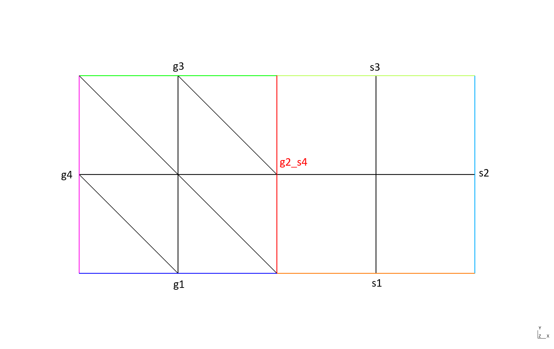
The following example shows the merging of two rectangles with different side names (mergeSharedBoundary set to true by default):
Rectangle R1(_xmin=0, _xmax=1, _ymin=0, _ymax=1, _nnodes={3,3},
             _domain_name="omega", _side_names={"g1","g2","g3","g4"});
Rectangle R2(_xmin=1, _xmax=2, _ymin=0, _ymax=1, _nnodes={3,3},
             _domain_name="omega", _side_names={"s1","s2","s3","s4"});
Mesh mR1P1(R1, _shape=_triangle, _order=1, _generator=_structured);
Mesh mR2Q1(R2, _shape=_quadrangle, _order=1, _generator=_structured);
Mesh mR1R2=merge(mR1P1,mR2Q1);
producing the domains:
Domain 'g1' of dimension 1 from mesh 'P1 mesh of [0,1]x[0,1] + Q1 mesh of [1,2]x[0,1]', orientation not computed, 2 elements
 geometric side element 13: side 3 of element 1
 geometric side element 14: side 3 of element 3
Domain 'g2_s4' of dimension 1 from mesh 'P1 mesh of [0,1]x[0,1] + Q1 mesh of [1,2]x[0,1]', orientation not computed, 2 elements
 geometric side element 29: side 2 of element 4, side 4 of element 9
 geometric side element 30: side 2 of element 8, side 4 of element 11
Domain 'g3' of dimension 1 from mesh 'P1 mesh of [0,1]x[0,1] + Q1 mesh of [1,2]x[0,1]', orientation not computed, 2 elements
 geometric side element 17: side 3 of element 6
 geometric side element 18: side 3 of element 8
Domain 'g4' of dimension 1 from mesh 'P1 mesh of [0,1]x[0,1] + Q1 mesh of [1,2]x[0,1]', orientation not computed, 2 elements
 geometric side element 19: side 2 of element 1
 geometric side element 20: side 2 of element 5
Domain 's1' of dimension 1 from mesh 'P1 mesh of [0,1]x[0,1] + Q1 mesh of [1,2]x[0,1]', orientation not computed, 2 elements
 geometric side element 21: side 1 of element 9
 geometric side element 22: side 1 of element 10
Domain 's2' of dimension 1 from mesh 'P1 mesh of [0,1]x[0,1] + Q1 mesh of [1,2]x[0,1]', orientation not computed, 2 elements
 geometric side element 23: side 2 of element 10
 geometric side element 24: side 2 of element 12
Domain 's3' of dimension 1 from mesh 'P1 mesh of [0,1]x[0,1] + Q1 mesh of [1,2]x[0,1]', orientation not computed, 2 elements
 geometric side element 25: side 3 of element 11
 geometric side element 26: side 3 of element 12
Domain 'omega' of dimension 2 from mesh 'P1 mesh of [0,1]x[0,1] + Q1 mesh of [1,2]x[0,1]', orientation not computed, 12 elements
 geometric element 6 (material 0, color 0, twin 0): triangle_Lagrange_1, orientation +0, linear map, measure = 0.125
 ...
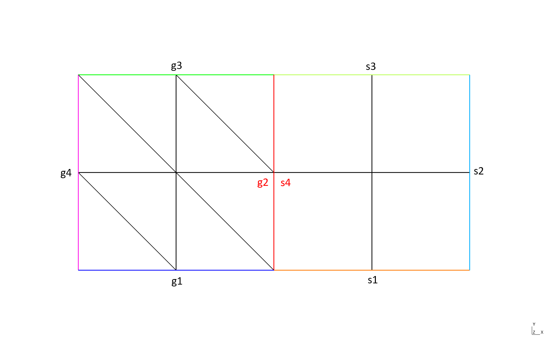
This is the same example but with mergeSharedBoundary set to false:
Mesh mR1R2=merge(mR1P1,mR2Q1, false);
producing the domains:
Domain 'g1' of dimension 1 from mesh 'P1 mesh of [0,1]x[0,1] + Q1 mesh of [1,2]x[0,1]', orientation not computed, 2 elements
 geometric side element 13: side 3 of element 1
 geometric side element 14: side 3 of element 3
Domain 'g2' of dimension 1 from mesh 'P1 mesh of [0,1]x[0,1] + Q1 mesh of [1,2]x[0,1]', orientation not computed, 2 elements
 geometric side element 15: side 2 of element 4
 geometric side element 16: side 2 of element 8
Domain 'g3' of dimension 1 from mesh 'P1 mesh of [0,1]x[0,1] + Q1 mesh of [1,2]x[0,1]', orientation not computed, 2 elements
 geometric side element 17: side 3 of element 6
 geometric side element 18: side 3 of element 8
Domain 'g4' of dimension 1 from mesh 'P1 mesh of [0,1]x[0,1] + Q1 mesh of [1,2]x[0,1]', orientation not computed, 2 elements
 geometric side element 19: side 2 of element 1
 geometric side element 20: side 2 of element 5
Domain 's1' of dimension 1 from mesh 'P1 mesh of [0,1]x[0,1] + Q1 mesh of [1,2]x[0,1]', orientation not computed, 2 elements
 geometric side element 21: side 1 of element 9
 geometric side element 22: side 1 of element 10
Domain 's2' of dimension 1 from mesh 'P1 mesh of [0,1]x[0,1] + Q1 mesh of [1,2]x[0,1]', orientation not computed, 2 elements
 geometric side element 23: side 2 of element 10
 geometric side element 24: side 2 of element 12
Domain 's3' of dimension 1 from mesh 'P1 mesh of [0,1]x[0,1] + Q1 mesh of [1,2]x[0,1]', orientation not computed, 2 elements
 geometric side element 25: side 3 of element 11
 geometric side element 26: side 3 of element 12
Domain 's4' of dimension 1 from mesh 'P1 mesh of [0,1]x[0,1] + Q1 mesh of [1,2]x[0,1]', orientation not computed, 2 elements
 geometric side element 27: side 4 of element 9
 geometric side element 28: side 4 of element 11
Domain 'omega' of dimension 2 from mesh 'P1 mesh of [0,1]x[0,1] + Q1 mesh of [1,2]x[0,1]', orientation not computed, 12 elements
 geometric element 2 (material 0, color 0, twin 0): triangle_Lagrange_1, orientation +0, linear map, measure = 0.125
 ...
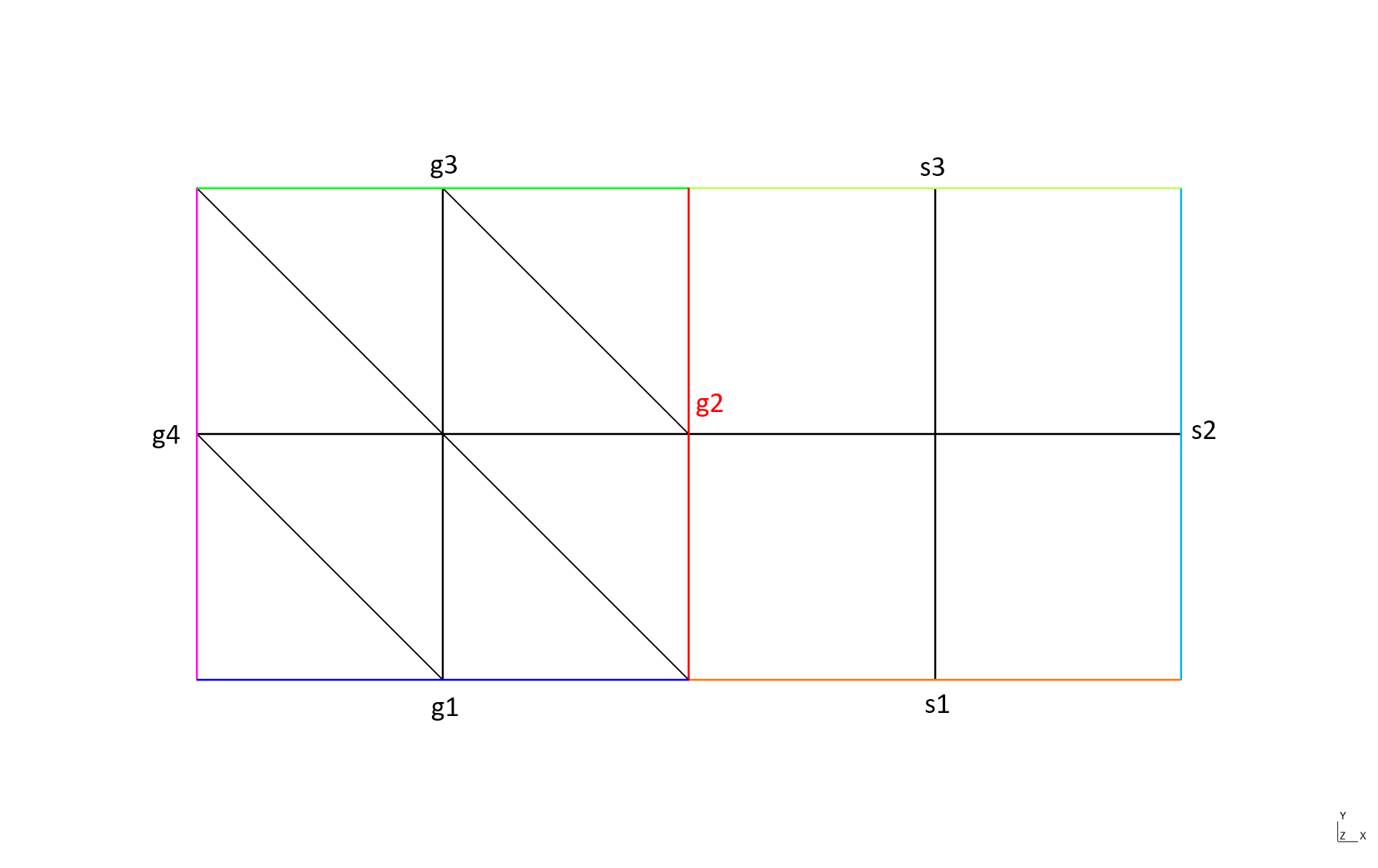
The case when the side domains defining the interface have the same name (here g2):
Rectangle R1(_xmin=0, _xmax=1, _ymin=0, _ymax=1, _nnodes={3,3},
             _domain_name="omega", _side_names={"g1","g2","g3","g4"});
Rectangle R2(_xmin=1, _xmax=2, _ymin=0, _ymax=1, _nnodes={3,3},
             _domain_name="omega", _side_names={"s1","s2","s3","g2"});
Mesh mR1P1(R1, _shape=_triangle, _order=1, _generator=_structured);
Mesh mR2Q1(R2, _shape=_quadrangle, _order=1, _generator=_structured);
Mesh mR1R2=merge(mR1P1,mR2Q1);
provides the following domains:
Domain 'g1' of dimension 1 from mesh 'P1 mesh of [0,1]x[0,1] + Q1 mesh of [1,2]x[0,1]', orientation not computed, 2 elements
 geometric side element 13: side 3 of element 1
 geometric side element 14: side 3 of element 3
Domain 'g2' of dimension 1 from mesh 'P1 mesh of [0,1]x[0,1] + Q1 mesh of [1,2]x[0,1]', orientation not computed, 2 elements
 geometric side element 29: side 2 of element 4, side 4 of element 9
 geometric side element 30: side 2 of element 8, side 4 of element 11
Domain 'g3' of dimension 1 from mesh 'P1 mesh of [0,1]x[0,1] + Q1 mesh of [1,2]x[0,1]', orientation not computed, 2 elements
 geometric side element 17: side 3 of element 6
 geometric side element 18: side 3 of element 8
Domain 'g4' of dimension 1 from mesh 'P1 mesh of [0,1]x[0,1] + Q1 mesh of [1,2]x[0,1]', orientation not computed, 2 elements
 geometric side element 19: side 2 of element 1
 geometric side element 20: side 2 of element 5
Domain 's1' of dimension 1 from mesh 'P1 mesh of [0,1]x[0,1] + Q1 mesh of [1,2]x[0,1]', orientation not computed, 2 elements
 geometric side element 23: side 1 of element 9
 geometric side element 24: side 1 of element 10
Domain 's2' of dimension 1 from mesh 'P1 mesh of [0,1]x[0,1] + Q1 mesh of [1,2]x[0,1]', orientation not computed, 2 elements
 geometric side element 25: side 2 of element 10
 geometric side element 26: side 2 of element 12
Domain 's3' of dimension 1 from mesh 'P1 mesh of [0,1]x[0,1] + Q1 mesh of [1,2]x[0,1]', orientation not computed, 2 elements
 geometric side element 27: side 3 of element 11
 geometric side element 28: side 3 of element 12
 Domain 'omega' of dimension 2 from mesh 'P1 mesh of [0,1]x[0,1] + Q1 mesh of [1,2]x[0,1]', orientation not computed, 12 elements
 geometric element 2 (material 0, color 0, twin 0): triangle_Lagrange_1, orientation +0, linear map, measure = 0.125
 ...
Finally, the case when all boundaries have the same name, except the interface:
Rectangle R1(_xmin=0, _xmax=1, _ymin=0, _ymax=1, _nnodes={3,3},
             _domain_name="omega", _side_names={"g","s","g","g"});
Rectangle R2(_xmin=1, _xmax=2, _ymin=0, _ymax=1, _nnodes={3,3},
             _domain_name="omega", _side_names={"g","g","g","s"});
Mesh mR1P1(R1, _shape=_triangle, _order=1, _generator=_structured);
Mesh mR2Q1(R2, _shape=_quadrangle, _order=1, _generator=_structured);
Mesh mR1R2=merge(mR1P1,mR2Q1);
provides the following domains:
Domain 'g' of dimension 1 from mesh 'P1 mesh of [0,1]x[0,1] + Q1 mesh of [1,2]x[0,1]', orientation not computed, 12 elements
 geometric side element 17: side 3 of element 6
 geometric side element 18: side 3 of element 8
 geometric side element 15: side 2 of element 1
 geometric side element 21: side 3 of element 11
 geometric side element 22: side 3 of element 12
 geometric side element 13: side 3 of element 3
 geometric side element 16: side 2 of element 5
 geometric side element 14: side 3 of element 1
 geometric side element 25: side 2 of element 12
 geometric side element 23: side 2 of element 10
 geometric side element 24: side 1 of element 10
 geometric side element 26: side 1 of element 9
Domain 's' of dimension 1 from mesh 'P1 mesh of [0,1]x[0,1] + Q1 mesh of [1,2]x[0,1]', orientation not computed, 2 elements
 geometric side element 29: side 2 of element 4, side 4 of element 9
 geometric side element 30: side 2 of element 8, side 4 of element 11
Domain 'omega' of dimension 2 from mesh 'P1 mesh of [0,1]x[0,1] + Q1 mesh of [1,2]x[0,1]', orientation not computed, 12 elements
 geometric element 6 (material 0, color 0, twin 0): triangle_Lagrange_1, orientation +0, linear map, measure = 0.125
 ...
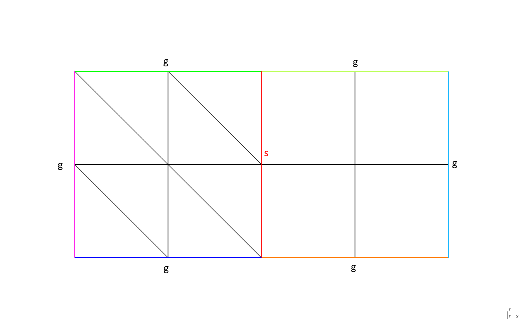
Note
As it can be seen in previous examples, an element of an interface domain handles two parent elements whereas an element of a side domain handles only one parent element. For continuous-FE computations, both types of domain can be used but sometimes it may
be important to work with the interface domain. Note that the member function updateParentOfSideElements transforms a side domain into an interface domain.
Various tools#
Some other tools are available build particular meshes.
Mesh of a regular cone-sphere
The GMSH tool does not produce satysfying mesh at the cone apex. This is the reason why it is provided a specific tool for meshing the surface of a cone-sphere based on mapping of triangle meshes to cone section or sphere section. A regular cone-sphere is a cone with a spherical cap with a regular (say C1) junction between the cone and the sphere. The following picture illustrates the meshing process:
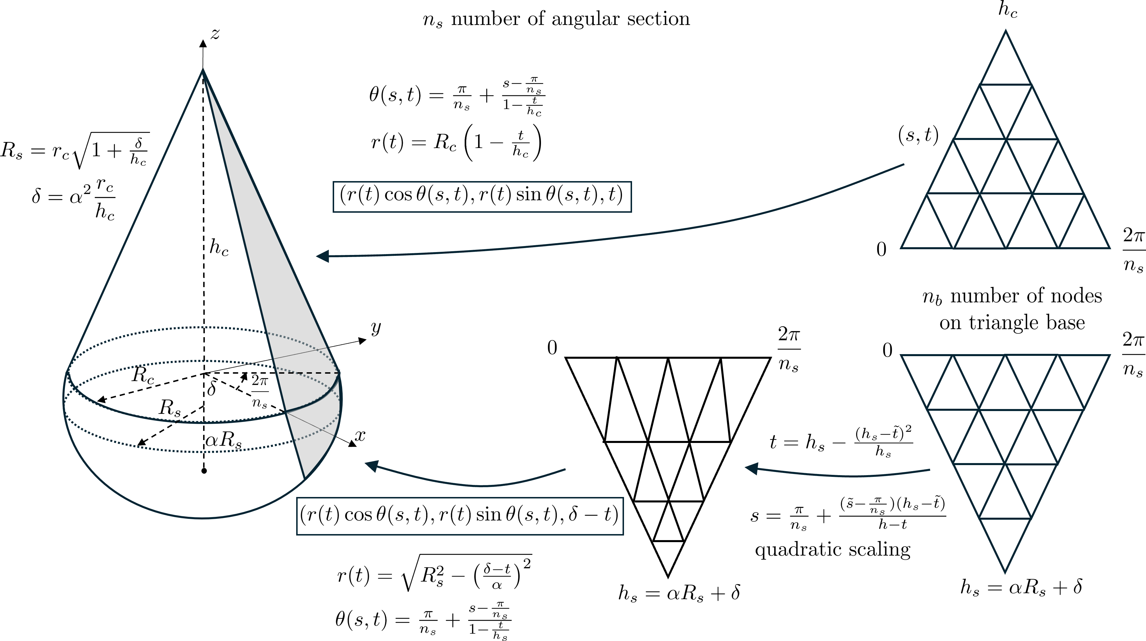
Mesh RegularConeSphereTri(Point c, Reals ax, Real hc, Real rc, Real obl, Number nbs, Number nbb, MeshGenerator mg, Strings domNames, String interfaceName, Strings apexNames)
where
cis the center of the cone basisaxis the cone axis vectorhcis the cone heightrcis the cone basis radiusoblis the oblateness \(\alpha\) of the sphere (1 means a sphere else an ellipsoid)nbsis the number of sections of sphere and conenbbis the number of nodes on the basis of section of cone or spheremgis the mesh generator to use (_subdiv or _gmsh)domNamesis the list of domain names to give to the cone and the ellipsoidinterfaceNameis the name of the interface between the cone and the ellipsoidapexNamesis the name of the cone apex and the sphere pole
For the sphere, there is a quadratic dilation along the meridians to avoid triangles that are too large at the sphere pole.
The following examples show how to use this function in the two cases of the subdivision generator and the gmsh generator:
Mesh meshConeSphere_subdiv = RegularConeSphereTri(Point(0.,0.,0.), Reals(0.,-1,0.), 4., 1, 0.5, 8, 17, _subdiv, Strings{"cone","sphere"},"circle",Strings{"apex","pole"});
Mesh meshConeSphere_gmsh   = RegularConeSphereTri(Point(0.,0.,0.), Reals(0.,-1,0.), 4., 1, 0.5, 8, 17, _gmsh, Strings{"cone","sphere"},"circle",Strings{"apex","pole"});
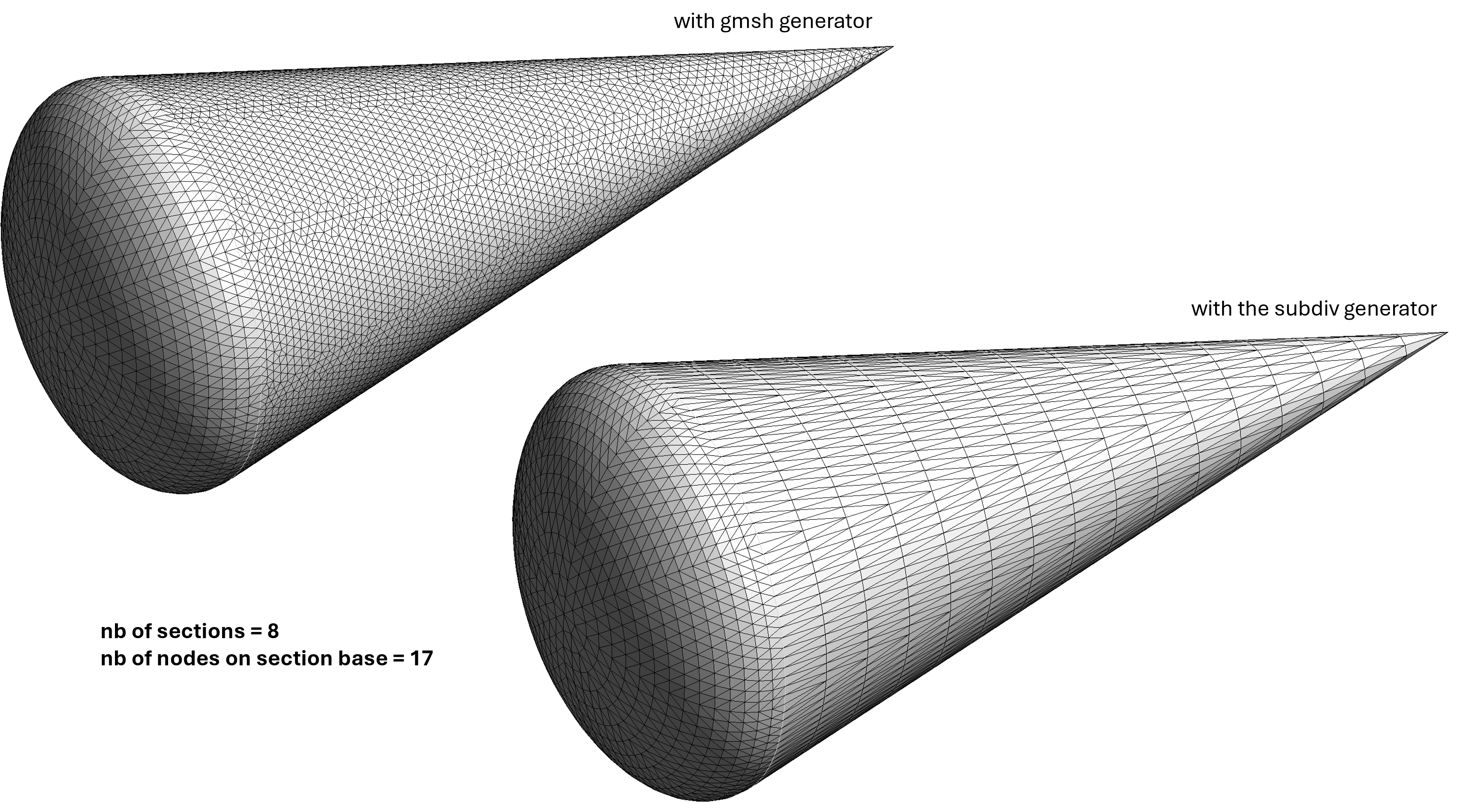
The mesh obtained with the subdivision generator is more regular than the mesh obtained with the gmsh generator, but the latter is more balanced because the number of nodes on cone sides is adjusted according to the mesh size on the cone basis. That is not possible with the subdivision generator! Note that only the surface is meshed with triangles, the volume is not meshed!
It may be of interest for advanced users to have a look on the code performing the cone mesh using the gmsh generator:
Triangle tri_c(_v1=Point(0.,0.,0.), _v2=Point(2*pn,0.,0.), _v3=Point(pn,hc,0.), _nnodes={nb,nl,nl}, _domain_name=nameCone, _side_names={edgename,"",""});
Mesh meshtri_c(tri_c, _order=1, _generator=_gmsh);
for (auto & v:meshtri_c.nodes) // map triangle to cone section
{
   real_t s=v[0], t=v[1];
   real_t theta=s, tn=t/hc;
   if (tn<1) theta=pn+(s-pn)/(1-tn);
   real_t r = rc*(1-tn);
   v = Point(r*std::cos(theta), r*std::sin(theta), t);
}
meshtri_c.changeDim(3);
Mesh mesh_cone=meshtri_c;
for (number_t k=0; k<ns-1;++k)
{
   Mesh meshtrik=rotate3d(meshtri_c, _axis=Reals(0.,0.,1.), _angle=2*pn*(k+1));
   mesh_cone.merge(meshtrik);
}
Cracking mesh#
Cracking a mesh means defining an interface between two domains as a crack; the nodes located on the crack are duplicated, one belonging to a domain and the second to the other domain (see ?).

