Splines#

Generally speaking, a spline is a piecewise polynomial curve that approaches, in a sense to be specified, an ordered list of points. The simplest one is the spline of degree 1 (linear spline) which connects the points by segments. XLiFE++ provides the Hermite cubic spline (C2), the Catmull-Row spline (C1), the B-spline and rational B-Spline (Ck) and the Bézier curve (Ck). The two first ones are interpolation splines while the last ones are approximation spline. Combining two rational B-splines in two directions gives a surface approximation, named NURBS acronym of Non Uniform Rational B-Spline.

C2 spline#

Let $(t_{i})_{0 \leq i \leq n}$ and $(y_{i})_{0 \leq i \leq n}$ . There exists a unique C2 piecewise cubic polynomial such that $q (t_{i}) = y_{i}$ for $0 \leq i \leq n$ and $q^{'} (t_{0}) = y_{0}^{'}, q^{'} (t_{n}) = y_{n}^{'}$ . Each cubic polynomial may be constructed from the knowledge of $b_{i} = q^{'} (t_{i}), 0 \leq i \leq n$ which is the solution of the following linear system ( $h_{i} = t_{i} - t_{i - 1}$ , $h_{i, j} = 2 (h_{i} + h_{j})$ ):

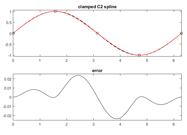
\begin{array}{r} [\begin{array}{ccccccc} 1 & 0 \\ h_{2} & h_{1, 2} & h_{1} \\ ⋱ & \dots & ⋱ \\ h_{i + 1} & h_{i, i + 1} & h_{i} \\ ⋱ & ⋱ & ⋱ \\ h_{n} & h_{n - 1, n} & h_{n - 1} \\ 0 & 1 \end{array}] \cdot [\begin{array}{c} b_{0} \\ b_{1} \\ ⋮ \\ b_{i} \\ ⋮ \\ b_{n - 1} \\ b_{n} \end{array}] = [\begin{array}{c} y_{0}^{'} \\ \frac{3}{h_{1} h_{2}} (h_{1}^{2} (y_{2} - y_{1}) \\ + h_{2}^{2} (y_{1} - y_{0})) \\ ⋮ \\ \frac{3}{h_{i} h_{i + 1}} (h_{i}^{2} (y_{i + 1} - y_{i}) + h_{i + 1}^{2} (y_{i} - y_{i - 1})) \\ ⋮ \\ \frac{3}{h_{n - 1} h_{n}} (h_{n - 1}^{2} (y_{n} - y_{n - 1}) + h_{n}^{2} (y_{n - 1} - y_{n - 2})) \\ y_{n}^{'} \end{array}] \end{array}

The spline is said to be clamped because derivatives at ends are imposed.

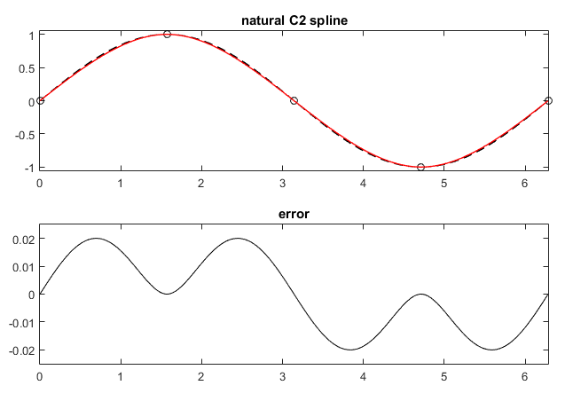
Other boundary conditions are usual : $q_{1}^{″} (t_{0}) = q_{n}^{″} (t_{n}) = 0$ leading to natural spline

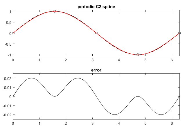
or periodicity conditions : $q_{1}^{'} (t_{0}) = q_{n}^{'} (t_{n})$ and $q_{1}^{″} (t_{0}) = q_{n}^{″} (t_{n})$ leading to periodic spline.

To interpolate any set of points $(P_{i})_{0 \leq i \leq n}$ in $R^{2}$ or $R^{3}$ , the previous method is extended as following. Let $T = (t_{i})_{0 \leq i \leq n}$ a set of parameters (knots) and a set of scalar values $Y = (y_{i})_{0 \leq i \leq n}$ , we denote $S_{T, Y}$ the spline function related to the sets $T, Y$ . The C2 spline related to the set of points (Pi) is defined as:

Q (t) = (S_{T, P^{1}} (t), S_{T, P^{2}} (t), S_{T, P^{3}} (t))

where $P^{k} = (P_{i}^{k})_{i = 0, n}$ with $P_{i}^{k}$ the $k^{t h}$ coordinate of the point $P_{i}$ .

The usual choices of parametrization are

the x-parametrization: $t_{i} = P_{i}^{1}, 0 \leq i \leq n$ (gives the original C2 spline).
the uniform parametrization: $t_{i} = i, 0 \leq i \leq n$ .
the chordal parametrization: $t_{0} = 0, t_{i} = t_{i - 1} + ‖ P_{i} - P_{i - 1} ‖, 1 \leq i \leq n$ .
the centripetal parametrization: $t_{0} = 0, t_{i} = t_{i - 1} + ‖ P_{i} - P_{i - 1} ‖^{\frac{1}{2}}, 1 \leq i \leq n$ .

Hint

To make the user life easier, the parameter is pullback to the interval $[0, 1]$ . In other words, user addresses the spline parametrization using $s \in [0, 1]$ that is mapped to $t = t_{0} + (1 - s) t_{n}$ where $t_{0}$ , $t_{n}$ are the spline parameter bounds . All splines work in the same way.

XLiFE++ provides the C2Spline class. There are two ways to construct a C2 spline, either by giving two vectors of reals $(T, Y)$ (classical C2 spline) or giving a vector of points $P$ (extended C2 spline). The following optional parameters may be given at construction:

the type of parametrization : one of _xParametrization, _uniformParametrization, _chordalParametrization, _centripetalParametrization
the boundary conditions : two of _naturalBC, _clampedBC, _periodicBC
the derivatives at end points (vector of reals) required when using clamped conditions

Number n=5;
Real x=0, dx=pi_/n;
vector<Point> points(n+1);
for(Number i=0;i<=n;i++, x+=dx) points[i]=Point(x,sin(x));
C2Spline csn(points,_xParametrization); //natural spline
C2Spline csc(points,_xParametrization,_clampedBC,_clampedBC,
Reals(1.,1.),Reals(1.,-1.)); //clamped spline
C2Spline csp(points, _xParametrization, _periodicBC); //periodic spline

Warning

When _xParametrization is selected, the curve is regarded as $x \mapsto y (x)$ curve and the returned “values” are 1D points. In contrast when an other parametrization is selected, the curve is regarded as $t \to (x (t), y (t))$ and the returned “values” are 2D points.

Warning

Be cautious with periodic conditions. For a periodic open curve (e.g $s i n x$ on $[0, 2 π]$ ) use only the _xParametrization mode and for a closed periodic curve use other parametrization mode.

Once a C2Spline object is constructed, using either the function evaluate or the operator (), it can be evaluated at any parameter $t \in [0, 1]$ .

...
C2Spline csn(points,_xParametrization);
Real t=0.5;            //midle parameter
Point P=csn(t);        //value
Point dP=csn(t,_dt);   //first derivative (vector as a point)
Point d2P=csn(t,_dt2); //second derivative (vector as a point)

C2Spline allocates also a Parametrization object related to the spline parametrization. Using this object, other quantities such as curvilinear abscissa, normal or tangent vector, curvatures are available (see The Parametrization class and Parametrization class):

...
C2Spline csn(points,_xParametrization);
Real t=0.5; //midle parameter
const Parametrization& pa=csn.parametrization();
Real c=pa.curvature(t);
Real s=pa.curabc(t);
Reals no=pa.normal(t);
Reals ta=pa.tangent(t);

Catmull-Rom spline#

Another way to construct interpolation spline consists in imposing also the tangent vectors $(T_{i})$ at control points $P_{i}$ . Several methods have been proposed and the Catmull-Rom method is one of them. On the interval $[t_{i}, t_{i + 1}]$ the spline $Q$ is defined by

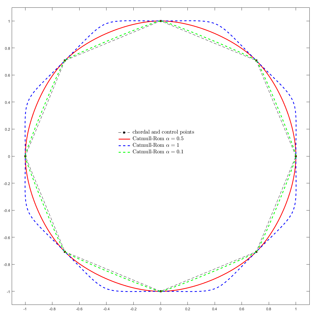
\begin{array}{r} Q (t) = [\begin{array}{cccc} 1 & t & t^{2} & t^{3} \end{array}] \cdot [\begin{array}{cccc} 0 & 1 & 0 & 0 \\ - α & 0 & α & 0 \\ 2 α & α - 3 & 3 - 3 α & - α \\ - α & 2 - α & α - 2 & α \end{array}] \cdot [\begin{array}{c} P_{i - 1} \\ P_{i} \\ P_{i + 1} \\ P_{i + 2} \end{array}] \end{array}

where $α$ is a tension parameter which is related to the underlying parametrization. The standard choices of $α$ are:

$α = 0$ : the standard Catmull-Rom spline,
$α = 1$ : the chordal Catmull-Rom spline,
$α = \frac{1}{2}$ : the centripetal Catmull-Rom spline.

The Catmull-Rom spline are local (moving a point modifies only the curve in the neighborhood of the point), the approximation is $C^{1}$ but not $C^{2}$ , the computation is fast. The centripetal Catmull-Rom spline has additional properties : there is no self-intersection, cusp will never occur and it follows the control points in a better way.

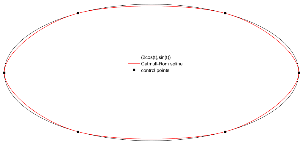
Note that to close a curve, it is sufficient to add the two last points at the beginning and the two first points at the end:

(P_{1} P_{2} P_{3} \dots P_{n - 2} P_{n - 1} P_{n}) \to (P_{n - 1} P_{n} P_{1} P_{2} P_{3} \dots P_{n - 2} P_{n - 1} P_{n} P_{1} P_{2})

and build Catmull-Rom spline on segments $[P_{n}, P_{1}, [P_{1}, P_{2},, \dots, [P_{n - 2}, P_{n - 1}], [P_{n - 1}, P_{n}]$ .

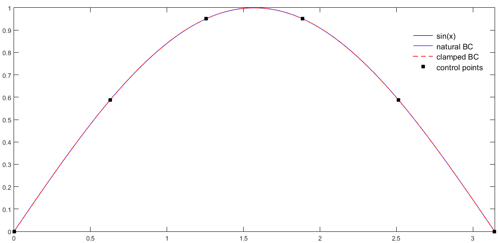
On the next figure, the influence of the parameter $α$ may be observed; the value $α = 0.5$ giving the best result.

XLiFE++ provides the CatmullRomSpline class. It has only one constructor from a vector of points $P$ and optional parameters are available:

the type of parametrization : one of _xParametrization , _uniformParametrization, _chordalParametrization, _centripetalParametrization
the tension parameter $α$ (default value: $0.5$ )
the boundary conditions : two of _undefBC, _naturalBC, _clampedBC, _periodicBC
the tangent vectors at end points (vector of reals) required when using clamped conditions

In this example, as the last point is the same as the first point, the curve will be automatically closed.

Once a CatmullRomSpline object is constructed, using either the function evaluate or the operator (), it can be evaluated at any parameter $t \in [0, 1]$

...
CatmullRomSpline cat(pts);
Real t=0.5             //midle parameter
Point P=cat(t);        //value
Point dP=cat(t,_dt);   //first derivative (vector as a point)
Point d2P=cat(t,_dt2); //second derivative (vector as a point)

CatmullRomSpline allocates also a Parametrization object related to the spline parametrization. Using this object, other quantities such as curvilinear abscissa, normal or tangent vector, curvatures are available (see The Parametrization class and Parametrization class):

...
CatmullRomSpline cat(pts);
Real t=0.5 //midle parameter
const Parametrization& pa=cat.parametrization();
Real c=pa.curvature(t);
Real s=pa.curabc(t);
Reals no=pa.normal(t);
Reals ta=pa.tangent(t);

Bézier curve#

For the set of control points $(P_{i}) 0 \leq i \leq n$ , the Bézier curve is defined by

Q (t) = \sum_{i = 0}^{n} B_{i}^{n} (t) P_{i} \forall t \in [0, 1]

where $B_{i}^{n} = C_{n}^{i} t^{i} (1 - t)^{n - i}$ are the Bernstein polynomials ( $\sum_{i = 0}^{n} B_{i} = 1)$ . Note that the degree of polynomials is equal to the number of points minus 1. There are the following properties

$Q_{0} = P_{0}$ and $Q_{1} = P_{n}$ but the curve does not interpolate the interior points $P_{1}, \dots, P_{n - 1}$
$P_{0} P_{1}$ (resp. $P_{n - 1} P_{n})$ is a tangent vector to the curve at $P_{0}$ (resp. $P_{n}$ ),
the curve is inside the convex hull of the control points,
the curve is $Ĉ^{\infty}$

XLiFE++ provides the BezierSpline class with only one simple constructor from a vector of points $P$ :

Number n=5;
vector<Point> points(n+1);
Real x=0, dx=pi_/n;
for(Number i=0;i<=n;i++, x+=dx) points[i]=Point(x,sin(x));
BezierSpline bz(points);

The parameter $t$ lives always in the interval $[0, 1]$ .

Once a BezierSpline object is constructed, using either the function evaluate or the operator (), it can be evaluated at any parameter $t \in [0, 1]$ :

...
BezierSpline bz(points);
Real t=0.5; //midle parameter
Point P=bz(t); //value
Point dP=bz(t,_dt); //first derivative (vector as a point)
Point d2P=bz(t,_dt2); //second derivative (vector as a point)

BezierSpline allocates also a Parametrization object related to the spline parametrization. Using this object, other quantities such as curvilinear abscissa, normal or tangent vector, curvatures are available (see The Parametrization class and Parametrization class):

...
BezierSpline bz(points);
Real t=0.5;
const Parametrization& pa=bz.parametrization();
Real c=pa.curvature(t);
Real s=pa.curabc(t);
Reals no=pa.normal(t);
Reals ta=pa.tangent(t)

B-Spline#

The B-spline curve is a generalization of the Bézier curve. Let $t_{0} \leq t_{1} \leq \dots \leq t_{m}$ a set of $m + 1$ knots and the B-spline functions of degree $k$ defined by recurrence:

\begin{array}{r} \begin{aligned} \forall 0 \leq i \leq m - 1 & B_{i, 0} (t) = {\begin{cases} 1 & t_{i} \leq t \leq t_{i + 1} \\ 0 & otherwise \end{cases} \\ \forall 1 \leq k \leq m - 1, 0 \leq i \leq m - k - 1 & B_{i, k} (t) = \frac{t - t_{i}}{t_{i + k} - t_{i}} B_{i, k - 1} (t) + \frac{t_{i + k + 1} - t}{t_{i + k + 1} - t_{i + 1}} B_{i + 1, k - 1} (t) \end{aligned} \end{array}

with the convention $\frac{∙}{0} = 0$ .

The B-spline functions have a lot of properties, in particular

$B_{i, k}$ is a polynomial of order $k$ on intervals $[t_{j}, t_{j + 1}]$ with support $[t_{i}, t_{i + k + 1}]$ ,
$0 < B_{i, k} < 1$ for $t \in [t_{i}, t_{i + k + 1}]$ ,
$B_{i, k}$ is $C^{\infty}$ at tight and is $C^{k - r}$ at knots of multiplicity $r$

For the set of $n + 1$ control points $P_{0}, P_{1}, \dots, P_{n}$ and the set of knots $t_{0} \leq t_{1} \leq \dots \leq t_{m}$ with $m \geq n + k + 1$ , the B-spline curve is defined by

Q (t) = \sum_{i = 0}^{n} B_{i, k} (t) P_{i} \forall t_{k} \leq t \leq t_{n + 1}

The B-spline curve is inside the convex hull of the control points, it is $C^{k - 1}$ if all the knots are of multiplicity 1, moving a point $P_{i}$ induces a modification of the points related to the interval $[t_{i}, t_{i + k}]$ . A Bézier curve is a B-Spline with a knots vector of the form $[0, 0, \dots, 0, 1, 1, \dots, 1]$ .

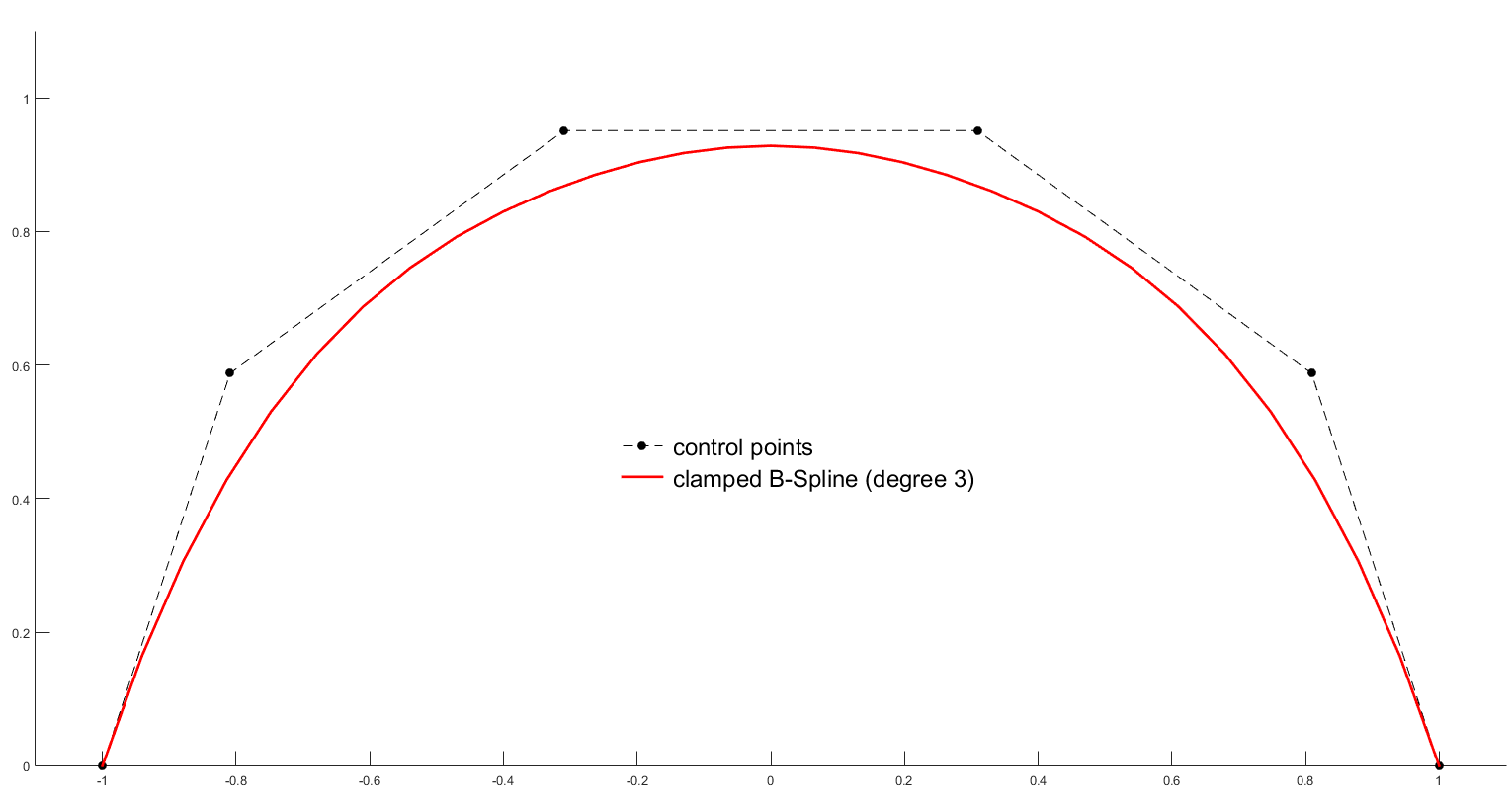
To clamp the curve at $P_{0}$ choose $t_{0} = t_{1} = \dots = t_{k} < t_{k + 1}$ and to close the curve duplicate the $k + 1$ first points at the end of the set of points.

$∙$ Clamped B-spline of degree 3 with 6 control points and knots $[0, 0, 0, 0, 1, 2, 3, 3, 3, 3]$ plotted on $[0, 3]$ :

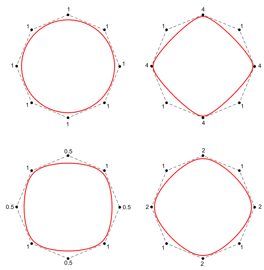
A rational B-spline is defined as following:

Q (t) = \frac{\sum_{i = 0}^{n} ω_{i} B_{i, k} (t) P_{i}}{\sum_{i = 0}^{n} ω_{i} B_{i, k} (t)} \forall t_{k} \leq t \leq t_{n + 1}

where $(ω_{i})_{i = 0, n}$ are some weights. When the weight $ω_{i}$ is large, the curve goes to the control point $P_{i}$ . When all the weights are equal to 1, the rational B-spline coincides with the B-spline.

if $t_{0} = t_{1} = \dots = t_{k} < t_{k + 1}$ and $P_{0} \neq P_{1}$ then

\begin{array}{r} \begin{array}{l} Q^{'} (t_{k}) = P_{0} \\ Q^{'} (t_{k}) = \frac{k}{t_{k + 1} - t_{k}} \frac{w_{1}}{w_{0}} (P_{1} - P_{0}) \\ Q^{'} (t_{k}) \times Q^{″} (t_{k}) = \frac{k^{2} (k - 1)}{(t k + 1 - t_{k})^{2} (t_{k + 2} - t_{k})} \frac{w_{1} w_{2}}{w_{0}^{2}} (P_{1} - P_{0}) \times (P_{2} - P_{0}), \\ κ = \frac{k - 1}{k} \frac{t_{k + 1} - t_{k}}{t_{k + 2} - t k} \frac{w_{1} w_{2}}{w_{0}^{2}} \frac{2 A}{c^{3}} (curvature) \end{array} \end{array}

with $A$ the surface of the triangle $(P_{0}, P_{1},, P_{2})$ and $c = ‖ P_{1} - P_{0} ‖$ . That gives a way to match the rational B-spline to another curve up to $C^{2}$ .

By solving a linear inverse problem, the control points may be calculated in order to interpolate a given set of points. In that case, the spline is named interpolation B-spline. For such spline, it is possible to impose the derivative vectors at the endpoints when the spline is clamped.

XLiFE++ provides the BSpline class with constructors that takes a vector of points $P$ and some optional data.

the type of B-spline, either _splineApproximation or _splineInterpolation
the degree of B-spline, default value 3
the type of parametrization : one of _uniformParametrization, _chordalParametrization, _centripetalParametrization
the boundary conditions : two of _undefBC , _naturalBC , _clampedBC , _periodicBC
derivative vectors at end points when clamped B-spline is selected
the vector of weights (default 1)

The given vector of points is either the list of control points (approximation B-spline) or the list of interpolation points (interpolation B-spline). When the type of B-spline is not given, it is assumed to be an approximation B-spline:

Number n=6;
vector<Point> pts(n+1);
Real s=0, ds=2*pi_/n;
for(Number i=0;i<=n;i++,s+=ds) pts[i]=Point(2*cos(s),sin(s)); //points on ellipse
Spline bs(points,3,_periodicBC);

Specifying a periodic condition at starting point stands obviously for periodic condition at ending point!

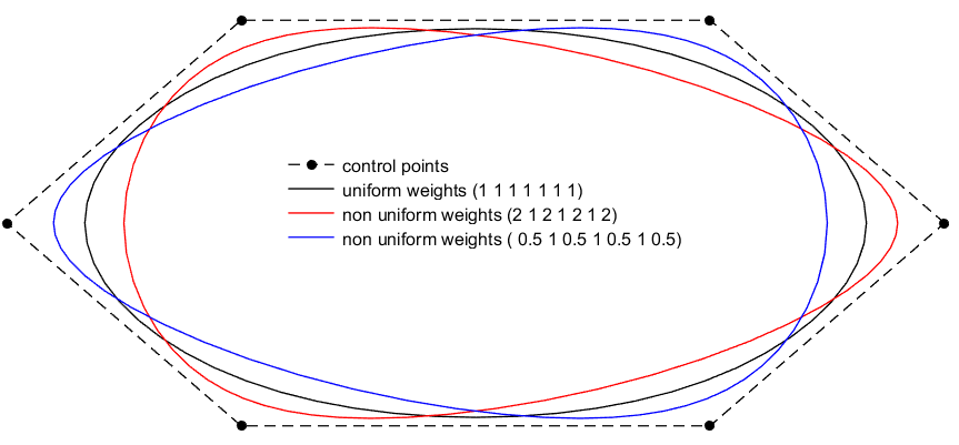
To use some weights, define a vector of weights of the size of vector of control points:

vector<Real> we(pts.size(),1.);
for(Number k=0;k<we.size();k+=2) we[k]=0.5;
BSpline bsw(pts,3,_periodicBC,_periodicBC,we);

Because of the signature of the constructor, both boundary conditions have to be specified even they are redundant!

Once a BSpline object is constructed, using either the function evaluate or the operator (), it can be evaluated at any parameter $t \in [0, 1]$ .

...
BSpline bs(points,3,_periodicBC);
Real t=0.5; //midle parameter
Point P=bs(t); //value
Point dP=bs(t,_dt); //first derivative (vector as a point)
Point d2P=bs(t,_dt2); //second derivative (vector as a point)

BSpline allocates also a Parametrization object related to the spline parametrization. Using this object, other quantities such as curvilinear abscissa, normal or tangent vector, curvatures are available (see The Parametrization class section and Parametrization class):

...
BSpline bs(points,3,_periodicBC);
Real t=0.5; //midle parameter
const Parametrization& pa=bs.parametrization();
Real c=pa.curvature(t);
Real s=pa.curabc(t);
Reals no=pa.normal(t);
Reals ta=pa.tangent(t);

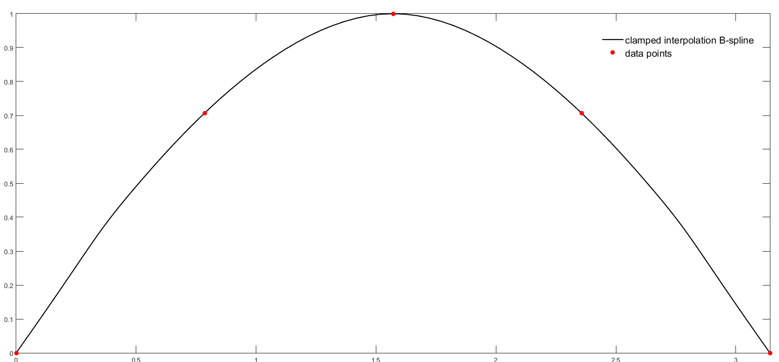
The following example shows how to build a clamped interpolation B-spline with a uniform parametrization from 5 points located on the sine curve:

...
vector<Point> pts(5,Point(0.,0.));
pts[1]=Point(pi_/4,sqrt(2)/2.);pts[2]=Point(pi_/2,1.);
pts[3]=Point(3*pi_/4,sqrt(2)/2.);pts[4]=Point(pi_,0.);
Reals d0(2,1.),d1=d0; d1[1]=-1.; //derivatives at end points
BSpline bs(_SplineInterpolation, pts, 3,_uniformParametrization, _clampedBC,_clampedBC,d0,d1);

When specifying only _splineInterpolation and a set of points in constructor, the B-spline will be a natural interpolation B-spline of degree 3 with a uniform parametrization (not rational).

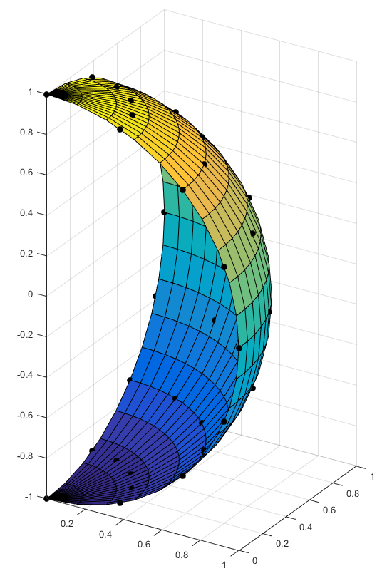
Spline surface (nurbs)#

The most common method to approximate surface are NURBS (non uniform rational B-spline) that are no more than the cross-product of two rational B-splines. Let

a set of $(m + 1) \times (n + 1)$ control points $P_{i j}, 0 \leq i \leq m$ and $0 \leq j \leq n$
a knot vector in u-direction and v-direction : $U = [u_{0}, u_{1}, \dots, u_{k}]$ and $V = [v_{0}, v_{1}, \dots, v_{l}]$
the degree $p$ in u-direction and the degree $q$ in v-direction
$k = m + p + 1$ and $l = n + q + 1$

The NURBS surface is defined by

(u, v) \to Q (u, v) = \frac{\sum_{i = 0}^{m} \sum_{j = 0}^{n} w_{i j} B_{i, p} (u) B_{j, q} (v) P_{i, j}}{\sum_{i = 0}^{m} \sum_{j = 0}^{n} w_{i j} B_{i, p} (u) B_{j, q} (u)}

To deal with nurbs, XLiFE++ provides the Nurbs class. There is only one constructor from a vector of vectors of points (control points) and optional parameters:

the degrees of B-spline along u /v parameter (default is 3)
the boundary conditions along $u / v$ parameter, for each parameter, two of _naturalBC, _clampedBC, _periodicBC
the vector of vectors of weights (default no weight)

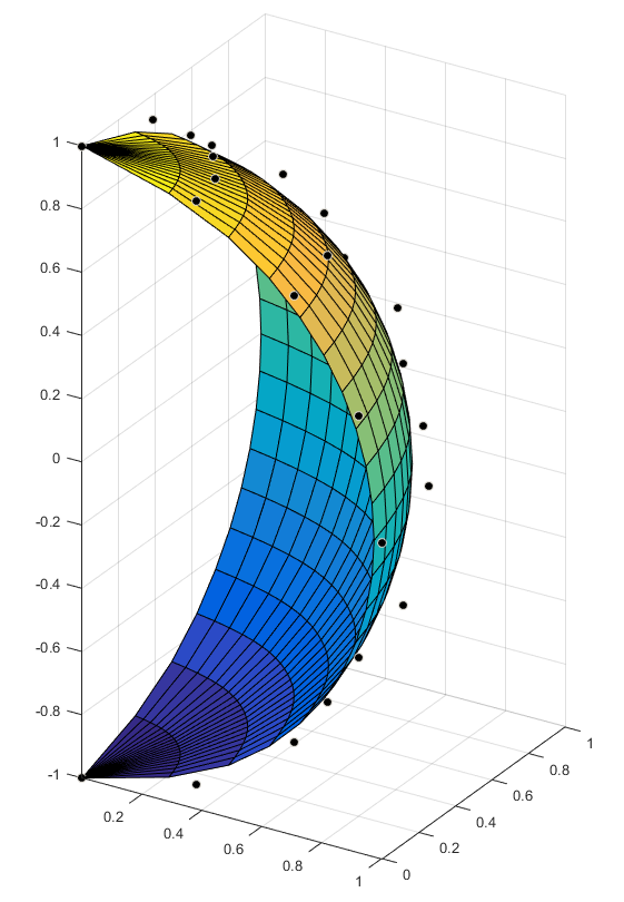
Number n=4;
Real ds=pi_/(2*n), u=-pi_/2, v=0;
PointMatrix pts(2*n+1,Points(n+1));
for(Number i=0;i<=2*n;i++,u+=ds) // points on the quarter of unit sphere
{
  v=0;
  for(Number j=0;j<=n;j++,v+=ds)
    pts[i][j]=Point(cos(u)*cos(v),cos(u)*sin(v),sin(u));
}
Nurbs nuA(_splineApproximation, pts); //create approximation nurbs
Nurbs nuI(_splineInterpolation, pts); //create interpolation nurbs

Once a Nurbs object is constructed, using either the function evaluate or the operator (), it can be evaluated at any parameter $(u, v) \in [0, 1] \times [0, 1]$ :

...
Point P=nu(0.5,0.5); //value
Point duP=nu(0.5,0.5,_d1); //first derivative (vector as a point)
Point dvP=nu(0.5,0.5,_d2); //first derivative (vector as a point)

Nurbs allocates also a Parametrization object related to the spline parametrization. Using this object, other quantities such as curvilinear abscissa, normal or tangent vector, curvatures are available (see The Parametrization class section and Parametrization class):

...
const Parametrization& pa=nu.parametrization();
Real u=0.5, v=0.5;
Reals cu=pa.curvatures(u,v); //two main curvatures
Reals no=pa.normal(u,v); //normal vector
Reals ta=pa.tangents(u,v); //two orthogonal tangent vectors in a same Vector