The Parametrization class#
Parametrizations are functions of interest in the context of geometry (2D/3D curve, 3D surface):
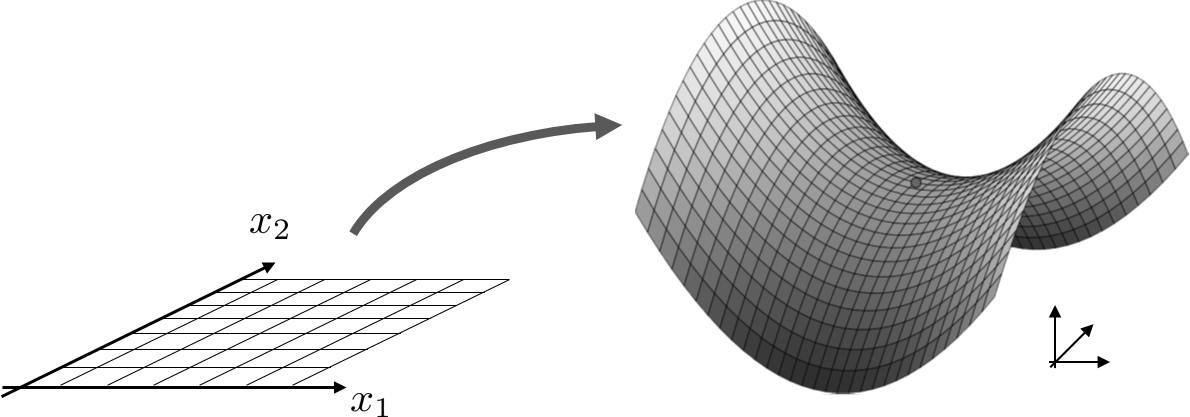
where x is the parameter (say t, or (u , v)) and \(p \le n\). When \(p=1\), parametrizations concern curves, when \(p=2\) parametrizations concerns surfaces. Note that p can be equal to n. In that case, f is a mapping (for instance the polar mapping).

Fig. 64 Surface parametrization#
XLiFE++ proposes the Parametrization class to handle such parametrization:
class Parametrization
{
 protected:
  Geometry* geom_p;       //pointer to the parametrized geometry (may be 0)
  Geometry* geomSupport_p;//pointer to the geometry support of the parameter
  par_fun f_p;            //pointer to the parametrization function with parameters
 public:
  String name;          //optionnal name useful for printing
  Dimen dimg;           //dimension of the geometry, set by init()
  Dimen dim;            //dimension of the arrival space, set by init()
  Number np=1000;       //number of points used to approximate curvilinear abcissa
  Parameters params;      //optional parameter list
  Real s0, s1;          //starting curvilinear abcissas (default 0)
  ContinuityOrder contOrder; //continuity order (by default _Cinf)
  par_fun curvature_p;    //pointer to a curvature function (may be 0)
  par_fun length_p;       //pointer to a length function (may be 0)
  par_fun invParametrization_p; //pointer to the inverse function (may be 0)
  par_fun normal_p;       //pointer to the normal function (may be 0)
  par_fun tangent_p;      //pointer to the tangent function (may be 0)
  par_fun curabc_p;       //pointer to the curvilinear abcissa function (may be 0)
  par_fun christoffel_p;  //pointer to the cristoffel symbols function (may be 0)
  ...
 }
par_fun is an alias of function of the form:
Vector<Real> fp(const Point& x, Parameters& pars, DiffOpType d);
where x is the parameter vector, pars a list of additional parameters (do not confuse with the parameter vector) and d a differential operator (one of _id, _d1, _d2, _d11, …) telling which derivative is requested.
The function f_p defining the parametrization function is mandatory while the other functions curvature_p, length_p, invParametrization_p, _normal_p, tangent_p, curabc_, christoffel_p are not. While these quantities can be calculated from the f_p function and its derivatives, it may be more efficient to provide specific functions to evaluate them. In particular, if the invParametrization_p is not provided, a Newton’s algorithm will be used to inverse the parametrization. This can be slow.
The geometry pointer geom_p optionnaly relates the parametrization to a Geometry object.
As a first example, consider the circle arc :
RealVector fc(const Point& x, Parameters& pars, DiffOpType d)
{
  Real R=pars("R"), t=x(1);
  if (d==_id) return RealVector(R*cos(t),R*sin(t));
  parfun_error("fc", d);
}
...
Parameters pars(1., "R");
Parametrization pc(-pi_/4, pi_/4, fc, pars, "arc");
To specify, for instance, the inverse of parametrization \(t=\mathrm{atan2}(x_2,x_1)\), do the following:
RealVector invfc(const Point& p, Parameters& pars, DiffOpType d)
{
  if (d!=_id) parfun_error("invfc",d);     // no derivative of inf
  return RealVector(1, atan2(p(2),t(1)));
}
...
Parametrization pc(-pi_/4, pi_/4, fc, pars, "arc");
pc.setinvParametrization(invfc);
Using setLength, setCurvature, setCurabc, setNormal, setTangent, other specific functions can be set.
When functions are quite simple, symbolic functions may be used:
Real R=1.;
Parametrization pc(-pi_/4, pi_/4, R*cos(x_1), R*sin(x_1), Parameters(), "arc");
In that case, an empty parameter is passed to the parametrization and R is passed
To construct parametrizations, the following syntaxes are available:
//1D parametrization on segment [a,b]
Parametrization pa(a, b, c++_fun, parameters, name);
Parametrization pa(a, b, symb_fun, symb_fun, parameters, name);
Parametrization pa(a, b, symb_fun, symb_fun, symb_fun, parameters, name);
//2D parametrization on rectangle[a,b]x[c,d]
Parametrization pa(a, b, c, d, c++_fun, parameters, name);
Parametrization pa(a, b, c, d, symb_fun, symb_fun, symb_fun, parameters, name);
//general constructors from any geometry support
Parametrization pa(geometry, c++_fun, parameters, name);
Parametrization pa(geometry, symb_fun, symb_fun, parameters, name);
Parametrization pa(geometry, symb_fun, symb_fun, symb_fun, parameters, name);
Once constructed, the Parametrization can compute the point at a parameter:
Parametrization pc(-pi_/4, pi_/4, cos(x_1), sin(x_1), Parameters(), "arc");
Point P=pc(pi_8);
Parametrization ps(-pi_/2,pi_/2,-pi_,pi_,cos(x_1)*cos(x_2),cos(x_1)*sin(x_2),
                   sin(x_1),Parameters(),"unit sphere");
Point Q=ps(0,0);
If derivatives or specific functions are available, it is also possible to compute some important geometrical quantities at parameter \(p\) (denoting \(f(p)=(f_1(p),f_2(p),[f_3(p)])\)):
-
the local lengths (ds)
for 1D parametrization (curve), the local “lengths” (ds) is defined as
\[ds(p)=\sqrt{(f'_1(p))^2+(f'_2(p))^2+[(f'_3(p))^2]}\]and for 2D parametrization (surface) the two “lengths” are defined as
\[\begin{split}ds_1(p)=\sqrt{(d_1f_1(p))^2+(d_1f_2(p))^2+(d_1f_3(p))^2}\\ ds_2(p)=\sqrt{(d_2f_1(p))^2+(d_2f_2(p))^2+(d_2f_3(p))^2}\end{split}\]RealVector Parametrization.lengths(p,[dif]) Real Parametrization.length(p,[dif]) Real Parametrization.bilength(p,[dif])
-
the curvatures (principal curvatures in 3D):
for 1D parametrization, the curvature is given by
\[c(p)=\frac{\|f''(p)\times f'(p)\|}{\|f'(p)\|^3}\]while for 2D parametrization (in \(\mathbb{R}^3\)), the main curvatures are the eigenvalues \((c_1(p),c_2(p))\) of the Weingarten’s matrix
\[\begin{split}W(p)=\frac{1}{EG-F^2} \left[ \begin{array}{cc} MF-LG & NF-LG\\ LF-ME & MF-NE \end{array}\right]\end{split}\]where \(E=(d_1f(p))^2\), \(F=d_1f(p)d_2f(p)\), \(G=(d_2f(p))^2\), \(L=d_{11}f(p).n\), \(M=2d_{12}f(p).n\), \(N=d_{22}f(p).n\). The Gauss curvature and the mean curvature are given by
\[c_G(p)=c_1(p)c_2(p) \mathrm{\ and\ } c_m(p)=\frac{1}{2}(c_1(p)+c_2(p)).\]RealMatrix Parametrization.weingarten(p) //only 3D surface RealVector Parametrization.curvatures(p,[dif]) Real Parametrization.curvature(p,[dif]) Real Parametrization.bicurvature(p,[dif]) //only 3D surface Real Parametrization.gaussCurvature(p,[dif]) //only 3D surface Real Parametrization.meanCurvature(p,[dif]) //only 3D surface Real Parametrization.normalCurvature(p,[dif]) //normal curvature rel. to d
-
the curvilinear abscissas (s)
The curvilinear abscissa is defined for 1D parametrization as \(p\) is a scalar:
\[\displaystyle s(p) =\int_0^p ds(t)\]and for 2D parametrization (\(p=(u,v)\)):
\[\displaystyle s_1(p)=\int_0^u ds_1(t,v)dt, \quad \displaystyle s_2(p)=\int_0^v ds_2(u,t)dt.\]RealVector Parametrization.curabcs(p,[dif]) Real Parametrization.curabc(p,[dif]) Real Parametrization.bicurabc(p,[dif]) //only 2D parametrization
-
the normal vector (N), the binormal vector (bN, only for 3D curve), the tangent vector (T) and the bitangent vector (b, only for 3D surface)
for 1D parametrization, the tangent vector is given by
\[T=\frac{f'(p)}{\|f'(p)\|}\]the first normal and the binormal (Frenet definition) by:
\[N=d_sT(p)/c(p)\mathrm{\ and\ } bN=T\times N.\]For 2D parametrization, the normal vector is given by
\[N=\frac{d_1f(p)\times d_2f(p) }{\|d_1f(p)\times d_2f(p))\|}\]and the tangent and bitangent vectors by:
\[T=\frac{d_1f(p)}{\|d_1f(p)\|} \mathrm{\ and\ } bT=T\times N.\]RealVector Parametrization.normals(p,[dif]) RealVector Parametrization.normal(p,[dif]) RealVector Parametrization.binormal(p,[dif]) //only 3D curve RealVector Parametrization.tangents(p,[dif]) RealVector Parametrization.tangent(p,[dif]) RealVector Parametrization.bitangent(p,[dif]) //only 3D surface
-
Other tools:
the torsion, only available for 3D curve :
\[\displaystyle \tau(p)=\frac{(f'(p),f''(p)\times f'''(p))}{\|f'(p)\times f''(p)\|}.\]the jacobian matrix (say \(J\)), the metric tensor (\(G=J^tJ\)), symmetric matrix stored as a 3[6]-vector:
\[(G_{11},G_{21},G_{22},[,G_{31},G_{32},,G_{33}])\]and the Christoffel symbols (immersed 2D surface, parametrized by \((u,v)\), stored as an 8-vector:
\[(\Gamma_{11}^1,\Gamma_{12}^1,\Gamma_{21}^1,\Gamma_{22}^1,\Gamma_{11}^2,\Gamma_{12}^2,\Gamma_{21}^2,\Gamma_{22}^2)\]Real Parametrization.torsion(p,[dif]) //only 3D curve RealMatrix Parametrization.jacobian(p,[dif]) RealVector Parametrization.metricTensor(p,[dif]) RealVector Parametrization.christoffel (p,[dif]) //only 3D surface
-
Inverse of the parametrization:
Point Parametrization.toParameter(Point);         //get parameter
Real Parametrization.toRealParameter(Point);      //get parameter (curve)
In previous functions dif is an optionnal argument taking as value either _id (default) or _d1, _d2, _d3 derivative operators whih are not fully operational.
These functions can take also, coordinates instead of Point, for instance:
RealVector Parametrization.lengths(x1,[x2],[dif])
Real Parametrization.length(x1,[x2],[dif])
Real Parametrization.bilength(x1,[x2],[dif])
Computations of most of these geometrical quantities require first and second derivatives of the parametrization. Only the computation of the torsion requires third derivatives. These derivatives are available when using symbolic functions but have to be handled when using a C++ function, for instance:
RealVector fc(const Point& x, Parameters& pars, DiffOpType d)
{
  Real R=pars("R"), t=x(1);
  switch (d)
  {
    case _id : return RealVector(R*cos(t), R*sin(t));   //no derivative
    case _d1 : return RealVector(-R*sin(t), R*cos(t));   //first derivative
    case _d11 : return RealVector(-R*cos(t), -R*sin(t)); //second derivative
    case _d111: return RealVector(R*sin(t), -R*cos(t)); //third derivative
    default : parfun_error("fc", d);
  }
  return RealVector();
}
Note that curvilinear abcissas are integrals. In XLiFE++, these integrals are approximated using a trapeze method with 1000 points and a linear interpolation.
This number of points may be changed using the np member data of Parametrization object:
Parametrization pc(-pi_/4, pi_/4, cos(x_1), sin(x_1), Parameters(), "arc");
pc.np = 500; // change the number of points of trapeze method
Note that it is also possible to associate C++ functions or symbolic functions to the lengths, the curvilinear abscissas, the normals, the tangents, the curvatures using the setLength, setCurabc, setNormal, setTangent, setCurvature functions. The inverse of the parametrization may be called if the user has given it either in C++ form or in symbolic form:
Note
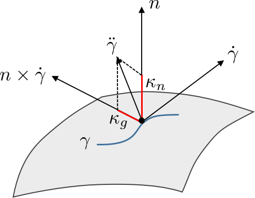
When dealing with curve on immersed surface \(s\rightarrow \gamma(s)=\varphi(u(s),v(s))\) (for instance a geodesic), the normal curvature at \(s\) is defined as (\(n\) a normal to the surface) :
Be careful, the sign of normal curvature depends on the choice of the surface normal. As the normal curvature depends only on the tangent \(d=\dot{\gamma}(s)\) of the curve at \(f(s)\), a more general tools is provided to compute the normal curvature at \(\varphi(u,v)\) relatively to the direction \(d\):
Real Parametrization.normalCurvature(p, d)  //normal curvature along d
RealVector Parametrization.curvatures(p,d) //Gauss,mean,normal curvature

Fig. 65 Normal curvature#
Up to now, the geodesic curvature \(\kappa_g\) is not available. Note that the curve curvature \(\kappa\) is related to the normal and geodesic curvatures by \(\kappa^2=\kappa_g^2+\kappa_n^2\).
All canonical geometries have an internal parametrization defined either on \([0,1]\) or \([0,1]\times[0,1]\) or \([0,1]\times[0,1]\times[0,1]\). See Geometry definition for the expression of the canonical parametrizations.
Piecewise parametrization#
When geometry is composite, the parametrization is managed by the PiecewiseParametrization class inheriting from Parametrization class.
The piecewise parametrization is the collection of “local” parametrizations related to canonical geometries that compose the composite geometry.
It is not globally \(C0\) but it is possible to travel through with the help of an additional map that handles the neighbor parametrizations. Most of geometrical functions are available.
class PiecewiseParametrization : public Parametrization
{
  public:
    vector<Point> vertices;
    map<Parametrization*,vector<Number>> vertexIndexes;
    map<Parametrization*, vector<pair<Parametrization*,Number>>> neighborParsMap;
  ...
};
with
The vertices vector collecting all the vertices (global numbering)
The vertexIndexes map collecting for each parametrization the local vertex numbers (relatively to global numbering)
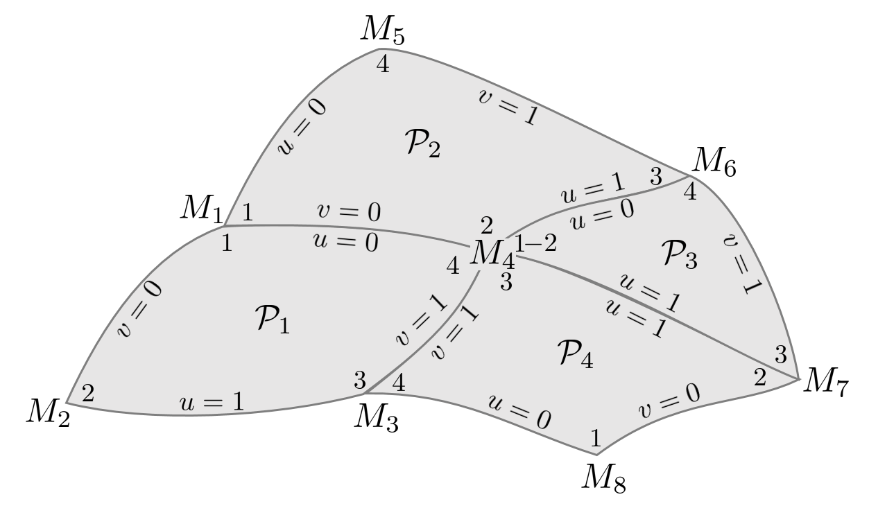
The neighborParsMap map collecting for each parametrization and each of its sides, the neighbor parametrization (if exists) and its relative side number (the side numbering being the following: side \(1\rightarrow v=0\), \(2\rightarrow u=1\), \(3\rightarrow v=1\) and \(4\rightarrow u=0\).

Fig. 66 Piecewise parametrization#
On the example made of surface patches:
The neighborParsMap map allows you to travel the piecewise parametrization by crossing patch interfaces. In 2D case, the piecewise parametrization is based on “quadrangular” patches, but they can be degenerated (triangular patches); but not fully degenerated (line). Note that this piecewise parametrization is not global \(C^0\). It is quite easy to produce a global \(C^0\) parametrization in 1D case, but it is another story in 2D case!
