
Integration methods#
To perform computation of integrals over elements, the library provides IntegrationMethod class which is an abstract class. Two abstract classes inherit from it: the SingleIM class to deal with single integral and the DoubleIM class to deal with double integral. All the classes have to inherit from these two classes.
Among integration methods, quadrature methods are general and well adapted to regular functions to be integrated.
XLiFE++ provides the QuadratureIM class, inherited from SingleIM class, which encapsulates the usual quadrature formulae defined in QuadratureIM class.
Besides, the ProductIM class, inherited from doubleIM class, manages a pair of SingleIM objects and may be used to take into double quadrature method (adapted to compute double integral with regular kernel).
In the case of double integrals, the integration method to be used can depend on the distance between two elements. This is the purpose of the IntegrationMethods which collects IntgMeth, which handles
an IntegrationMethod object and additional parameters, including a distance criterion and a function part if it is split into a regular and a singular part.
The dependency diagram looks like


Note that
SauterSchwabIMclass is dedicated to compute double integrals involving Laplace/Helmholtz kernel in 3d for any kind of finite elementDuffyIMclass is dedicated to compute double integrals involving Laplace/Helmholtz kernel in 2d for any kind of finite elementLenoirSalles2dIM,LenoirSalles3dIM,LenoirSalles2dIRandLenoirSalles3dIRare dedicated to compute double or single integral involving Laplace/Hemholtz kernel and are working only with P0 or P1 Lagrange element.CollinoIMclass is dedicated to compute double integrals involving Maxwell kernel in 3d and Raviart-Thomas element of order 0FilonIMclass computes 1d oscillatory integrals \(\int_0^T f(t)e^{-iat}\).
The IntegrationMethod class#
The IntegrationMethod class, basis class of all integration methods, manages general information about them:
class IntegrationMethod
{
  public:
    String name;                  // name for doc purpose
    IntegrationMethodType imType; // method type (see below)
    SingularityType singularType; // singularity supported (_notsingular, _r, _logr, _loglogr)
    real_t singularOrder;         // singularity order
    string_t kerName;             // kernel shortname if adapted to (default is empty)
    bool requireRefElement;       // true if method require reference element (false)
    bool requirePhyElement;       // true if method require physical element (false)
    bool requireNormal;           // true if method involves normal (false)
};
Up to now, the types of integral defined in enumeration are:
enum IntegrationMethodType
{
  _undefIM, _quadratureIM, _polynomialIM, _productIM,
  _LenoirSalles2dIM, _LenoirSalles3dIM, _LenoirSalles2dIR, _LenoirSalles3dIR,
  _SauterSchwabIM, _SauterSchwabSymIM, _DuffyIM, _DuffySymIM,
  _HMatrixIM, _CollinoIM, _FilonIM
};
Note
Except the first four types, all the types _xxxIM are aliased xxx, for instance SauterSchwab is an alias of _SauterSchwabIM.
The _HMatrixIM method type is a very particular case because it is used to choose the hierarchical matrix representation (HMatrix class) and compression methods which can be seen
in some way as an integration method! See H-matrices.
The SingleIM, DoubleIM inherited from the IntegrationMethod are purely interface classes to real integration methods for single or double integral.
The QuadratureIM class#
The QuadratureIM class is dedicated to integration methods adapted to integrals of regular functions, based on quadrature points and quadrature weights.
It is derived from SingleIM class and mainly handles a list of Quadrature objects indexed by ShapeType to deal with multiple quadrature rule
in case of domain having more than one shape type. As the quadrature rule are often involved in context of FE computation, the Quadrature class may store shape values:
class QuadratureIM : public SingleIM
{public:
  QuadRule quadRule;         // QuadRule to be used (may be _defaultRule)
  Number degree;             // degree of quadrature (default 3)
  map<ShapeType,Quadrature*> quadratures_; // to store Quadrature obj for different shapes
  map<ShapeType,vector<ShapeValues>*> shapevalues_; // to store shape values
  ...
}
This class offers the setQuadrature and setQuadratures functions
that set the Quadrature objects according to the shapes, the quadrature rule and the order provided.
The Quadrature and the QuadratureRule classes#
The quadrature formulae have the following form:
where \((\widehat{x}_i)_{i=1,q}\) are quadrature points belonging to reference element \(\hat{E}\) and \((\omega_i)_{i=1,q}\) are quadrature weights.
The Quadrature class manages all information related to quadrature :
class Quadrature
{
  public:
    GeomRefElement* geomRefElt_p;  // pointer to geometric reference element
    QuadratureRule quadratureRule; // embedded QuadratureRule object
    QuadRule rule;                 // type of quadrature rule
    number_t degree;               // degree of quadrature rule
    bool hasPointsOnBoundary;      // as it reads
    string_t name;                 // name of quadrature formula (for doc purposes)
    static std::vector<Quadrature*> theQuadratureRules; //global list of Quadrature
    ...
};
where
geomRefElt_prefers to the geometry (segment, triangle, …) bearing the quadrature.quadratureRulerefers to aQuadratureRuleobject which handles the points and weights of quadrature and the functions to build them.-
rulerefers to aQuadRulewhich is an enumeration of all types of quadrature supported:enum QuadRule { _defaultRule = 0, _GaussLegendreRule, _symmetricalGaussRule, _GaussLobattoRule, _nodalRule, _miscRule, _GrundmannMollerRule, _doubleQuadrature, _evenGaussLegendreRule, _evenGaussLobattoRule };
degree_is either the degree of the quadrature rule or the degree of the polynomial interpolation in case of nodal quadrature rules.the static vector
theQuadraturescollects all the pointers toQuadratureobject in order to have only one instance of aQuadratureobject.
The practical “construction” of a Quadrature object is done by the external function findQuadrature which first, searches in the static vector theQuadratures the quadrature defined by a shape, a quadrature rule and a degree.
If it is not found, a new Quadrature object is created on the heap. In any case a pointer to the Quadrature object is returned.
This class offers also the bestQuadrule function that returns the “best” quadrature rule regarding the shape and the degree.
The QuadratureRule class stores the quadrature points and quadrature weights and provides member functions to load them :
class QuadratureRule
{
  std::vector<Real> coords_;  // point coordinates of quadrature rule
  std::vector<Real> weights_; // weights of quadrature rule
  Dimen dim_;                 // dimension of points
  ...
};
The main task of this class is to load quadrature points and weights. Thus, there are a lot of member functions to load these values. Some of them have a general purpose (for instance to build quadrature rules from tensor or conical products of 1D rules) and others are specific to one quadrature rule.
Here is a simple example of how to use quadrature objects :
Quadrature* q=findQuadrature(_triangle, _GaussLegendreRule, 3);
Real S=0, x,y;
Number k=0;
for (Number i =0; i<q->quadratureRule.size(); i++,k+=2)
{
  x=q->quadratureRule.coords()[k];
  y=q->quadratureRule.coords()[k+1];
  S+=q->quadratureRule.weights()[i]*std::sin(x*y);
}
std::cout << "S=" << S;
Up to now, there exist quadrature formulae for unit segment \(]0,1[\), for unit triangle, for unit quadrangle (square), for unit tetrahedron, for unit hexahedron (cube) for unit prism and for unit pyramid. The following tables give the list of available quadrature formulae:
Gauss-Legendre |
Gauss-Lobatto |
Grundmann-Muller |
symmetrical Gauss |
|
|---|---|---|---|---|
segment |
any odd degree |
any odd degree |
||
quadrangle |
any odd degree |
any odd degree |
any odd degree up to 21 |
|
triangle |
any odd degree |
any odd degree |
degree up to 10 |
|
hexahedron |
any odd degree |
any odd degree |
odd degree up to 11 |
|
tetrahedron |
any odd degree |
any odd degree |
degree up to 10 |
|
prism |
degree up to 10 |
|||
pyramid |
any odd degree |
any odd degree |
degree up to 10 |
nodal |
miscellaneous |
|
|---|---|---|
segment |
P1 to P4 |
|
quadrangle |
Q1 to Q4 |
|
triangle |
P1 to P3 |
Hammer-Stroud 1 to 6 |
hexahedron |
Q1 to Q4 |
|
tetrahedron |
P1, P3 |
Stroud 1 to 5 |
prism |
P1 |
centroid 1, tensor product 1,3,5 |
pyramid |
P1 |
centroid 1, Stroud 7 |
More precisely, the rules that are implemented:
-
1D rules
Gauss-Legendre rule, degree \(2n+1\), \(n\) points
Gauss-Lobatto rule, degree \(2n-1\), \(n\) points
Gauss-Lobatto rule, degree \(2n-1\), \(n\) points
trapezoidal rule, degree \(1\), \(2\) points
Simpson rule, degree \(3\), \(3\) points
Simpson \(3\) \(8\) rule, degree \(3\), \(4\) points
Boole rule, degree \(5\), \(5\) points
Wedge rule, degree \(5\), \(6\) points
-
Rules over the unit simplex (less quadrature points BUT with negative weights)
TN Grundmann-Moller rule, degree \(2n+1\), \(C^n_{n+d+1}\) points
-
Rules over the unit triangle \(\{ x > 0, y >0, x+y < 1 \}\)
T2P2 MidEdge rule
T2P2 Hammer-Stroud rule
T2P3 Albrecht-Collatz rule, degree \(3\), \(6\) points, Stroud (p.314)
T2P3 Stroud rule, degree \(3\), \(7\) points, Stroud (p.308)
T2P5 Radon-Hammer-Marlowe-Stroud rule, degree \(6\), \(7\) points, Stroud (p.314)
T2P6 Hammer rule, degree \(6\), \(12\) points, G.Dhatt, G.Touzot (p.298)
Gauss-Legendre (conical product), any order
symmetrical Gauss up to degree 10
-
Rules over the unit quadrangle \([0,1]\times[0,1]\)
nodal degree 1 to 4 (1D nodal, tensor product)
Gauss-Legendre (tensor product), any order
Gauss-Lobatto (tensor product), any order
-
Rules over the unit tetrahedron \(\{x > 0, y >0, z>0, x+y+z < 1\}\)
T3P2 Hammer-Stroud rule, degree 2, 4 points, Stroud (p.307)
T3P3 Stroud rule, degree \(3\), \(8\) points, Stroud (p.308)
T3P5 Stroud rule, degree \(5\), \(15\) points, Stroud (p.315)
Gauss-Legendre (conical product), any order
symmetrical Gauss up to degree 10
-
Rules over the unit hexahedron \([0,1]\times[0,1]\times[0,1]\)
nodal degree 1 to 4 (1D nodal, tensor product)
Gauss-Legendre (tensor product), any order
Gauss-Lobatto (tensor product), any order
symmetrical Gauss up to degree 11
-
Rules over the unit prism \(\{ 0 < x, y < 1, x+y<1, 0 < z < 1\}\)
P1 nodal rule
tensor product of 2-points Gauss-Legendre rule on [0,1] and Stroud 7 points formula on the unit triangle (degree 3)
tensor product of 3-points Gauss-Legendre rule on [0,1] and Radon-Hammmer-Marlowe-Stroud 7 points formula on the unit triangle (degree 5)
Gauss-Legendre (tensor product), any order
Gauss-Lobatto (tensor product), any order
symmetrical Gauss up to degree 10
-
Rules over the unit pyramid \(\{ 0 < x, y < 1-z, 0 < z < 1\}\)
P1 nodal rule
symmetrical Gauss up to degree 10
-
Rules built from lower dimension rules
tensor product of quadrature rules (quadrangle and hexahedron)
conical product of quadrature rules (triangle and pyramid)
rule built from 1D nodal rule which are quadrangle nodal rule
rule built from 1D nodal rule which are hexahedron nodal rule
References:
F.D. Witherden and P.E. Vincent. On the identification of symmetric quadrature rules for finite element methods. Computers & Mathematics with Applications, 69(10):1232–1241, 2015. URL: https://www.sciencedirect.com/science/article/pii/S0898122115001224, doi:https://doi.org/10.1016/j.camwa.2015.03.017.
G Dhatt. The finite element method displayed. Wiley, Chichester [West Sussex] ; New York, 1984. ISBN 0471901105.
Axel Grundmann and H. M. Möller. Invariant integration formulas for the n-simplex by combinatorial methods. SIAM Journal on Numerical Analysis, 15(2):282–290, 1978. URL: https://doi.org/10.1137/0715019, arXiv:https://doi.org/10.1137/0715019, doi:10.1137/0715019.
A.H. Stroud. Approximate calculation of multiple integrals. Prentice-hall series in automatic computation. Prentice-Hall, Englewood Cliffs, 1971. ISBN 0130438936.
To choose quadrature rules, the class provides the static function bestQuadRule returning the ‘best’ quadrature rule for a given shape \(S\) and a given polynomial degree \(d\).
static QuadRule bestQuadRule(ShapeType, Number);
“Best rule” has to be understood as the rule on shape \(S\) with the minimum of quadrature points integrating exactly polynomials of degree \(d\).
The following tables gives the current best rules:
degree |
quadrature rule |
order |
number of quadrature points |
|---|---|---|---|
\(2n\), \(2n+1\) |
Gauss-Legendre |
\(2n+1\) |
\(n+1\) |
degree |
quadrature rule |
order |
number of quadrature points |
|---|---|---|---|
\(1\) |
Gauss-Legendre |
\(1\) |
\(1\) |
\(2\), \(3\) |
Gauss-Legendre |
\(3\) |
\(4\) |
\(4\), \(5\) |
Symmetrical Gauss |
\(5\) |
\(8\) |
\(6\), \(7\) |
Symmetrical Gauss |
\(7\) |
\(12\) |
\(8\), \(9\) |
Symmetrical Gauss |
\(9\) |
\(20\) |
\(10\), \(11\) |
Symmetrical Gauss |
\(11\) |
\(28\) |
\(12\), \(13\) |
Symmetrical Gauss |
\(13\) |
\(37\) |
\(14\), \(15\) |
Symmetrical Gauss |
\(15\) |
\(48\) |
\(16\), \(17\) |
Symmetrical Gauss |
\(17\) |
\(60\) |
\(18\), \(19\) |
Symmetrical Gauss |
\(19\) |
\(72\) |
\(20\), \(21\) |
Symmetrical Gauss |
\(21\) |
\(85\) |
\(2n\), \(2n+1\), \(n \geq 11\) |
Gauss-Legendre |
\(2n+1\) |
\({(n+1)}^2\) |
degree |
quadrature rule |
order |
number of quadrature points |
|---|---|---|---|
\(1\) |
centroid rule |
\(1\) |
\(1\) |
\(2\) |
P2 Hammer-Stroud |
\(2\) |
\(2\) |
\(3\) |
Grundmann-Moller |
\(3\) |
\(3\) |
\(4\) |
Symmetrical Gauss |
\(4\) |
\(6\) |
\(5\) |
Symmetrical Gauss |
\(5\) |
\(7\) |
\(6\) |
Symmetrical Gauss |
\(6\) |
\(12\) |
\(7\) |
Symmetrical Gauss |
\(7\) |
\(15\) |
\(8\) |
Symmetrical Gauss |
\(8\) |
\(16\) |
\(9\) |
Symmetrical Gauss |
\(9\) |
\(19\) |
\(10\) |
Symmetrical Gauss |
\(10\) |
\(25\) |
\(11\) |
Symmetrical Gauss |
\(11\) |
\(28\) |
\(12\) |
Symmetrical Gauss |
\(12\) |
\(33\) |
\(13\) |
Symmetrical Gauss |
\(13\) |
\(37\) |
\(14\) |
Symmetrical Gauss |
\(14\) |
\(42\) |
\(15\) |
Symmetrical Gauss |
\(15\) |
\(49\) |
\(16\) |
Symmetrical Gauss |
\(16\) |
\(55\) |
\(17\) |
Symmetrical Gauss |
\(17\) |
\(60\) |
\(18\) |
Symmetrical Gauss |
\(18\) |
\(67\) |
\(19\) |
Symmetrical Gauss |
\(19\) |
\(73\) |
\(20\) |
Symmetrical Gauss |
\(20\) |
\(79\) |
\(21\) |
Gauss-Legendre |
\(21\) |
\(132\) |
\(2n\), \(2n+1\), \(n \geq 11\) |
Gauss-Legendre |
\(2n+1\) |
\((n+1) (n+2)\) |
degree |
quadrature rule |
order |
number of quadrature points |
|---|---|---|---|
\(1\) |
Gauss-Legendre |
\(1\) |
\(1\) |
\(2\), \(3\) |
Symmetrical Gauss |
\(3\) |
\(6\) |
\(4\), \(5\) |
Symmetrical Gauss |
\(5\) |
\(14\) |
\(6\), \(7\) |
Symmetrical Gauss |
\(7\) |
\(34\) |
\(8\), \(9\) |
Symmetrical Gauss |
\(9\) |
\(58\) |
\(10\), \(11\) |
Symmetrical Gauss |
\(11\) |
\(90\) |
\(2n\), \(2n+1\), \(n\geq 6\) |
Gauss-Legendre |
\(2n+1\) |
\({(n+1)}^3\) |
degree |
quadrature rule |
order |
number of quadrature points |
|---|---|---|---|
\(1\) |
centroid rule |
\(1\) |
\(1\) |
\(2\) |
P2 Hammer-Stroud |
\(2\) |
\(4\) |
\(3\) |
Grundmann-Moller |
\(3\) |
\(5\) |
\(4\), \(5\) |
Symmetrical Gauss |
\(5\) |
\(14\) |
\(6\) |
Symmetrical Gauss |
\(6\) |
\(24\) |
\(7\) |
Symmetrical Gauss |
\(7\) |
\(35\) |
\(8\) |
Symmetrical Gauss |
\(8\) |
\(46\) |
\(9\) |
Symmetrical Gauss |
\(9\) |
\(59\) |
\(10\) |
Symmetrical Gauss |
\(10\) |
\(81\) |
\(11\) |
Grundmann-Moller |
\(11\) |
\(126\) |
\(2n\), \(2n+1\) |
Grundmann-Moller |
\(2n+1\) |
\(\binom{n+4}{4}\) |
degree |
quadrature rule |
order |
number of quadrature points |
|---|---|---|---|
\(1\) |
centroid rule |
\(1\) |
\(1\) |
\(2\) |
Symmetrical Gauss |
\(2\) |
\(5\) |
\(3\) |
Symmetrical Gauss |
\(3\) |
\(8\) |
\(4\) |
Symmetrical Gauss |
\(4\) |
\(11\) |
\(5\) |
Symmetrical Gauss |
\(5\) |
\(16\) |
\(6\) |
Symmetrical Gauss |
\(6\) |
\(28\) |
\(7\) |
Symmetrical Gauss |
\(7\) |
\(35\) |
\(8\) |
Symmetrical Gauss |
\(8\) |
\(46\) |
\(9\) |
Symmetrical Gauss |
\(9\) |
\(60\) |
\(10\) |
Symmetrical Gauss |
\(10\) |
\(85\) |
degree |
quadrature rule |
order |
number of quadrature points |
|---|---|---|---|
\(1\) |
centroid rule |
\(1\) |
\(1\) |
\(2\) |
Symmetrical Gauss |
\(2\) |
\(5\) |
\(3\) |
Symmetrical Gauss |
\(3\) |
\(6\) |
\(4\) |
Symmetrical Gauss |
\(4\) |
\(10\) |
\(5\) |
Symmetrical Gauss |
\(5\) |
\(15\) |
\(6\) |
Symmetrical Gauss |
\(6\) |
\(24\) |
\(7\) |
Symmetrical Gauss |
\(7\) |
\(31\) |
\(8\) |
Symmetrical Gauss |
\(8\) |
\(47\) |
\(9\) |
Symmetrical Gauss |
\(9\) |
\(62\) |
\(10\) |
Symmetrical Gauss |
\(10\) |
\(83\) |
How to add a new quadrature formula ?#
To add a new quadrature formula, say myRule on a unit element, say geomelt:
first, add myRule to
QuadRuleenumeration typenext, add in
QuadratureRuleclass the member function defining the quadrature points and weights, e.gQuadratureRule::myQuadRule.finally, modify the geomeltQuadrature function by adding in the right case statement the properties of the new quadrature formula. For instance, in the case of a new quadrature formula on the triangle:
Quadrature* triangleQuadrature(QuadRule rule, number_t numb)
{
  ...
  switch (appliedRule)
  {
    case _nodalRule: ...; break;
    case ...
    case _myRule:
      q=findQuadrature(_triangle, _myRule, numb, false); //find if already loaded
      if (q==nullptr) // create new Quadrature
      {
        q=new Quadrature(_triangle, _myRule,numb,"my rule",false);
        q->quadratureRule.myQuadRule(numb); //set points and weights
      }
      break;
  default: badDegreeRule(numb,"miscellaneous rule", _triangle); break;
 }
 ...
 return q;
}
Attention
When the QuadRule enumeration is modified, the dictionaries and may be, the Quadrature::bestQuadRule static function must be updated.
The ProductIM class#
In order to represent a product of integration method over a product of geometric domain (double integrals), the ProductIM class carries two SingleIM pointers:
class ProductIM : public DoubleIM
{
  protected:
    SingleIM* im_x; // integration method along x
    SingleIM* im_y; // integration method along y
};
ProductIM objects are used to calculate double integrals involving kernels which are regular on the integration domain.
Integration methods for singular kernels#
To deal with single or double integral involving a kernel with a singularity on the integration domain, say
XLiFE++ provides some additional classes:
DuffyIM(segments) andSauterSchwabIM(triangle) well adapted to Laplace/Helmholtz kernel and any regular functions \(p1\), \(p2\)LenoirSalles2dIM(segments) andLenoirSalles3dIM(triangles) well adapted to Laplace kernel with \(p1\), \(p2\) constant or linear functionsCollinoIM(triangles) designed to Maxwell 3d BEM integrals using Raviart-Thomas elements (affine).LenoirSalles2dIR(segments) andLenoirSalles3dIR(triangles) well adapted to calculate integral representation invoving Laplace kernel with \(p1\), \(p2\) constant or linear functions
DuffyIM class#
This class deals with double integral over segments (\(S_1\times S_2\)) involving 2d kernel \(K\) with \(\log|x-y|\) singularity.
For adjacent elements (sharing only one vertex) a Duffy transform is used (segments \([S_1,S_2]\) and \([T_1,T_2]\) with \(T_1=S_1\)):
For self influence (\(S_1=S_2\)) two methods are proposed:
-
one based on a splitting of the unit square \(]0,1[\times]0,1[\) in \(n_y\) decreasing rectangles
\[]0,1[\times]\frac{1}{2^k},\frac{1}{2^{k-1}}[,\ k=1,n-1 \text{ and } ]0,1[\times]0,\frac{1}{2^{n-1}}[.\] one based on diagonal splitting and using a \(t^p\) transform in order to concentrate the quadrature points in the neighbor of the diagonal \(x=y\) (for more details see the separate documentation quadrature_self_influence_2D). This is the default one with \(p=5\).
class DuffyIM : public DoubleIM
{
  public:
  Quadrature* quadSelfX, *quadSelfY; // quadratures on segment [0,1] for self influence
  Quadrature* quadAdjtX, *quadAdjtY; // quadratures on segment [0,1] for adjacent elements
  Number ordSelfX, ordSelfY;         // order of quadratures for self influence
  Number ordAdjtX, ordAdjtY;         // order of quadratures for adjacent elements
  Number selfOrd;                    // order of t^p transform or number of number of layers(def=5)
  bool useSelfTrans;                 // use improved method for self influence (def=true)

  DuffyIM(IntegrationMethodType);    // default constructor
  DuffyIM(Number oX=6, Number oY=6); // full constructor
  DuffyIM(QuadRule qsX, Number osX, QuadRule qsY, Number osY, QuadRule qaX, Number oaX, QuadRule qaY, Number oaY, Number so=5, bool ust=true);
  DuffyIM(const Quadrature&);        // full constructor from a quadrature
}
The class provides computation functions regarding geometrical configuration of segments:
template<typename K>
 void computeIE(...) const;
 void SelfInfluences(...) const;
 void SelfInfluencesTP(...) const;
 void AdjacentSegments(...) const;
 void k4(...) const;
 void k5(...) const;
The computation precision is very sensitive to the order of quadrature used in y direction. When using the first method to compute the self influence coefficients, to get very accurate results in the case of P2 mesh, very high order quadrature must be involved, for instance
DuffyIM dufim(_GaussLegendreRule,60, _GaussLegendreRule,60, _GaussLegendreRule,60, _GaussLegendreRule,60,5,false);
which lead to 300 quadrature points in each direction for self-influence coefficients!
Using the second method improves drastically the efficiency of the computation :
DuffyIM dufim(_GaussLegendreRule, 30, _GaussLegendreRule, 30, _GaussLegendreRule, 50, _GaussLegendreRule, 50, 5, true);
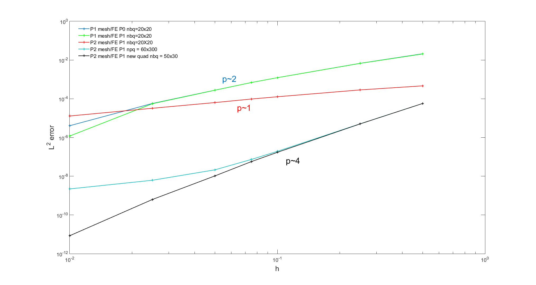
The following picture shows the convergence rates of the BEM (single layer) in case of the diffraction (\(k=1.35\)) of a plane wave on a disk (radius 1). It can be noted that with a very low quadrature (red curve) the convergence rate is not captured at all, with a very high quadrature using the first method (cyan curve) the convergence rate becomes hard to capture when refining the mesh and finally the second method (black curve) allows well capturing the convergence rate with a reasonable number of quadrature points.
SauterSchwabIM class#
This class deals with double integral over triangles involving 3d kernel \(K\) with \(|x-y|^{-1}\) singularity, say
class SauterSchwabIM : public DoubleIM
{
 public:
  Quadrature* quadSelf;    //quadrature for self influence
  Quadrature* quadEdge;    //quadrature for elements adjacent by edge
  Quadrature* quadVertex;  //quadrature for elements adjacent by vertex
  Number ordSelf;        //order of quadrature for self influence
  Number ordEdge;        //order of quadrature for edge adjacence
  Number ordVertex;      //order of quadrature for vertex adjacence

  SauterSchwabIM(Number =3); //basic constructor (order 3)
  SauterSchwabIM(Quadrature&); //full constructor from quadrature object
}
LenoirSalles2dIM and LenoirSalles3dIM classes#
The LenoirSalles2dIM class can compute analytically
where \(p_1\) and \(p_2\) are either the P0 or P1 shape functions on segments \(S_1\) and \(S_2\) and the LenoirSalles3dIM class computes analytically
where \(p_1\) and \(p_2\) are the P0 shape functions (say \(1\)) on triangles \(T_1\) and \(T_2\).
These two classes have no member data and only one basic constructor.
LenoirSalles2dIR and LenoirSalles3dIR classes#
The LenoirSalles2dIR class can compute analytically
where \(p\) is either the P0 or P1 shape functions on segment \(S\) and the LenoirSalles3dIR class that computes analytically
where \(p\) is the P0 or P1 shape functions on triangle \(T\).
These two classes have no member data and only one basic constructor.
All the previous classes provides, a clone method, access to the list of quadratures if there are ones and an interface to the computation functions:
virtual LenoirSalles2dIM* clone() const;  //covariant
virtual std::list<Quadrature*> quadratures() const; //list of quadratures
template<typename K>
void computeIE(const Element* S, const Element* T, AdjacenceInfo& adj, const KernelOperatorOnUnknowns& kuv, Matrix<K>& res, IEcomputationParameters& iep, Vector<K>& vopu, Vector<K>& vopv, Vector<K>& vopk) const;
CollinoIM class#
The CollinoIM class is a wrapper to an integration method developed by F. Collino to deal with some integrals involved in 3D Maxwell BEM when using Raviart-Thomas elements of order 1 (triangle). More precisely, it can compute the integrals:
and
where \((w_i)_{i=1,n}\) denote the Raviart-Thomas shape functions and \(H(k;x,y)\) the Green function of the Helmholtz equation (wave number k) in the 3D free space. The class looks like
enum ComputeIntgFlag {_computeI1=1, _computeI2, _computeBoth};

class CollinoIM : public DoubleIM
{
 private:
  myquad_t* quads_;
public:
 Number ordSNear; //default 12
 Number ordTNear; //default 64
 Number ordTFar;  //default 3
 Real eta;        //default 3.
 ComputeIntgFlag computeFlag;

 CollinoIM();
 CollinoIM(ComputeIntgFlag cf, Number otf, Number otn, Number osn, Real e);
 CollinoIM(const CollinoIM&);
 ~CollinoIM();
 virtual CollinoIM* clone() const;
 CollinoIM& operator=(const CollinoIM&);

 virtual std::list<Quadrature*> quadratures() const;
 virtual void print(std::ostream& os) const;
 template<typename K>
 void computeIE(const Element*, const Element*, AdjacenceInfo&, const KernelOperatorOnUnknowns&, Matrix<K>&, IEcomputationParameters&,Vector<K>&,Vector<K>&,Vector<K>&) const;
}
quads_ is a pointer to a quadrature structure provided by the Collino package, ordSNear, ordTNear, ordTFar are order of quadrature rules used, eta is a relative distance used to separate far and near triangle interactions and computeFlag allows you to choose the integrals that have to be computed. computeIE is the main computation function calling the real computation function (ElemTools_weakstrong_c) provided by the Collino package (see files {itshape Collino.hpp} and Collino.cpp).
The IntegrationMethods class#
The IntegrationMethods class collects some IntgMeth objects that handle an integration method pointer with some additional parameters:
class IntgMeth
{
  public:
   const IntegrationMethod* intgMeth;
   FunctionPart functionPart; //_allFunction, _regularPart, _singularPart
  Real bound;              //bound value
}
The bound value may be used to select an integration method regarding a criterion. For instance, in BEM computation the criterion is the relative distance between the centroids of elements. Besides, using functionPart member, different integration method may be called on different part of the kernel, see Kernel class. This class has only some constructors and print stuff:
IntgMeth(const IntegrationMethod& im, FunctionPart fp=_allFunction, Real b=0);
IntgMeth(const IntgMeth&);
~IntgMeth();
IntgMeth& operator=(const IntgMeth&);
void print(std::ostream&) const;
void print(PrintStream&) const;
friend ostream& operator<<(ostream&, const IntgMeth&)
For safe multi-threading behavior, copy constructor and assign operator do a full copy of IntegrationMethod object.
The IntegrationMethods class is simply a vector of IntMeth object:
class IntegrationMethods
{
 public:
  vector<IntgMeth> intgMethods;
  typedef vector<IntgMeth>::const_iterator const_iterator;
  typedef vector<IntgMeth>::iterator iterator;
 ...
}
This class provides many constructors depending on the number of integration methods given (up to 3 at this time), to some shortcuts :
IntegrationMethods() {};
IntegrationMethods(const IntegrationMethod&,FunctionPart=_allFunction,Real=0);
...
void add(const IntegrationMethod&, FunctionPart=_allFunction,Real=0);
void push_back(const IntgMeth&);
To handle more than 3 integration methods, use the add member function.
Besides, the class offers some accessors and print stuff:
const IntgMeth& operator[](Number) cons ;
vector<IntgMeth>::const_iterator begin() const;
vector<IntgMeth>::const_iterator end() const;
vector<IntgMeth>::iterator begin();
vector<IntgMeth>::iterator end();
bool empty() const {return intgMethods.empty();}
void print(ostream&) const;
void print(PrintStream&) const;
friend ostream& operator<<(ostream&, const IntegrationMethods&);
In BEM computation, the following relative distance between two elements (\(E_i\), \(E_j\)) is used:
So defining for instance
IntegrationMethods ims(SauterSchwabIM(4), 0., symmetrical_Gauss, 5, 1., symmetrical_Gauss, 3);
the BEM computation algorithm will perform on function (all part):
Sauter-Schwab with quadrature of order 4 on segment |
if \(dr(E_i,E_j)=0\) |
Symmetrical gauss quadrature of order 5 on triangle |
if \(0 < dr(E_i,E_j) \leq 1\) |
Symmetrical gauss quadrature of order 3 on triangle |
if \(dr(E_i,E_j) > 1\) |
Standard integration method#
Classic 1d integration methods#
For various integration purpose, XLiFE++ provides the uniform rectangle, trapeze and Simpson method (\(h=\frac{b-a}{n}\)):
with \(f\) a real or complex function. The rectangle method integrates exactly P0 polynomials, the trapeze method integrates exactly P1 polynomials whereas the Simpson method integrates exactly P3 polynomials. They respectively approximate the integral with order 1, 2 and 3.
For each of them, four template functions (with names rectangle, trapz, simpson) are provided according to the user gives the values of \(f\) on a uniform set of points, the function \(f\) or a function \(f\) with some parameters (e.g. trapeze method):
template<typename T, typename Iterator>
T trapz(Number n, Real h, Iterator itb, T& intg);
template<typename T>
T trapz(const std::vector<T>& f, Real h);
T trapz(T(*f)(Real), Real a, Real b, Number n);
T trapz(T(*f)(Real, Parameters&), Parameters& pars, Real a, Real b, Number n);
XLiFE++ provides also an adaptive trapeze method using the improved trapeze method (\(0.25(b-a)(f(a)+2f((a+b)/2)+f(b))\)) to get an estimator. The user has to give its function (with parameters if required), the integral bounds a tolerance factor (\(10^{-6}\) if not given):
template<typename T>
T adaptiveTrapz(T(*f)(Real), Real a, Real b, Real eps=1E-6);
T adaptiveTrapz(T(*f)(Real,Parameters&), Parameters& pars, Real a, Real b, Real eps=1E-6)
Hint
Because at the first step, the adaptive method uses 5 points uniformly distributed, the result may be surprising if unfortunately the function takes the same value at these points!
Discrete Fast Fourier Transform (FFT)#
XLiFE++ provides the standard 1D discrete fast Fourier transform with \(2^n\) values:
FFT and inverse FFT are computed using some functions addressing iterators on a collection of real or complex values:
template<class Iterator>
void  fft(Iterator ita, Iterator itb, Number log2n);
void ifft(Iterator ita, Iterator itb, Number log2n);
Computations from real or complex vectors is also available, but the results are always some complex vectors:
template<typename T>
vector<Complex>& fft(vector<T>& f, vector<Complex>& g);
vector<Complex>& ifft(vector<T>& f, vector<Complex>& g);
The following example shows how to use them:
Number ln=6, n=64;
Vector<Complex> f(n),g(n),f2(n);
for (Number i=0; i<n; i++) f[i]=std::sin(2*i*pi_/(n-1));
fft(f.begin(),g.begin(),ln);
ifft(g.begin(),f2.begin(),ln); //f2 should be very close to f
// or
fft(f,g); ifft(g,f2);
Integration methods for oscillatory integrals#
Up to now, only one method is provided to compute 1D oscillatory integrals based on the Filon’s method. The Filon’s method XLiFE++ proposes is designed to compute an approximation of the following oscillatory integral:
where \(f\) is a slowly varying function with real or complex values (template type).
Considering a uniform grid \(t_n=n\,dt,\ \forall n=0,N\) and an interpolation space on this grid, say \(\text{vect }(w_n)_{n=0,N}\) where \(w_n\) are polynomial on each segment \([t_{n-1},t_n]\); the Filon’s method consists in interpolating the function \(f\):
Substituting \(f\) by its interpolation in integral and collecting terms in a particular way, the integral \(I(x)\) is thus approximated as follows:
where \(Cj(x)\) and \(C'_j\) are coefficients of the form :math:` int_0^1 tau_j(s) exp^{-i,x,s,dt}ds` with \(\tau_j\) some shape functions on the segment \([0,1]\) ant \(t_n^j\) the support of the \(j^{th}\) DoF on the segment \([t_{n-1},t_n]\). The second sum in \(I_N\) appears only when using Hermite interpolation; for Lagrange interpolation, \(C'_j(x)=0\).
If the values \(f(t_n^j)_{n=0,N}\) and \(f'(t_n^j)_{n=0,N}\) (if Hermite interpolation) are pre-computed, the computation of \(I_N(x)\) for many values of \(x\) may be very efficient!
The FilonIMT is a template class, FilonIM being its complex specialization:
template <typename T = Complex>
class FilonIMT : public SingleIM
{
 typedef T(*funT)(Real);  // T function pointer alias
 protected:
  Number ord_;        //interpolation order of (0,1 or 2)
  Real tf_;           //upper bound of integral (lower bound is 0)
  Real dt_;           //grid step if uniform
  Number ns_;         //number of segments
  Vector<T> fn_;        //values of f (and df if required) on the grid
  Vector<Real> tn_;   //grid points
  ...
}
ord_ corresponds to the interpolation used : 0 for Lagrange P0, 1 for Lagrange P1 and 2 for Hermite P3. The values \(f(t_n^j)_{n=0,N}\) and \(f'(t_n^j)_{n=0,N}\) are collected (only one copy) in the same vector with the following storage:
Lagrange P0 : \(f(dt/2) f(3\,dt/2),\,\dots\, f((N-1/2)dt)\) (\(N\) values)
Lagrange P1 : \(f(0) f(dt),\,\dots\, f(N\,dt)\) (\(N+1\) values)
Hermite P3 : \(f(0) f'(0) f(dt) f'(dt),\,\dots\, f(N\,dt) f'(N\,dt)`\) (\(2(N+1)\) values)
The FilonIMT class provides several constructors that pre-compute the values of \(f\) and \(f'\) from user’s functions of the real variable with real or complex values. More precisely, the following types are available:
Real f(Real t) {...}
Complex f(Real t) {...}
Real f(Real t, Parameters& pars) {...}
Complex f(Real t, Parameters& pars) {...}
It is also possible to construct a FilonIMT object passing the values of \(f\) at uniformly distributed points on:math:` [0,t_f]`. In that case, Filon of order 1 is selected. So the class looks like
typedef T(*funT)(Real);
typedef T(*funTP)(Real, Parameters& pa);
FilonIMT();
FilonIMT(Number o,Number N,Real tf,funT f);
FilonIMT(Number o,Number N,Real tf,funT f,funT df);
FilonIMT(Number o,Number N,Real tf,funTP f,Parameters& pars);
FilonIMT(Number o,Number N,Real tf,funTP f,funTP df, Parameters& pars);
FilonIMT(const Vector<T>& vf, Real tf);
void init(Number N,funT f,funT df);
void init(Number N,funTP f,funTP df,Parameters& pars);
Number size() const {return tn_.size();}     //grid size
template <typename S>
Complex coef(const S& x, Number j) const;  //Filon's coefficients
Complex compute(const S& x) const;           //compute I(x)
Complex operator()(const S& x) const         //compute I(x)
virtual void print(std::ostream& os) const;    //print FilonIMT on stream
This class is quite easy to use, for instance to compute the integral
by the P1-Filon method:
Complex f(Real x) {return Complex(std::exp(-x),0.);}
...
FilonIM fim(1, 100, 10, f);
Complex y = fim(0.5);
// or in a more compact syntax if only one evaluation
Complex y = FilonIM(1, 100, 10, f)(0.5);
To invoke Hermite P3 Filon method, define also the derivative of \(f\):
Complex f(Real x)  {return Complex(exp(-x),0.);}
Complex df(Real x) {return Complex(-exp(-x),0.);}
...
FilonIM fim(2, 100, 10, f, df);
Complex y = fim(0.5);
Hint
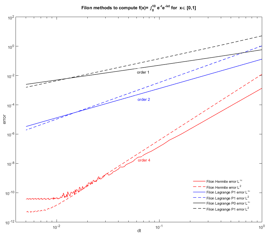
The P0 Filon method is of order 1, the P1 Filon is of order 2 while the Hermite P3 Filon is of order 4. The Hermite P3 Filon is less stable than the Lagrange Filon methods!
See also
library= finiteElements,
header= Quadrature.hpp QuadratureRule.hpp IntegrationMethod.hpp,
implementation= Quadrature.cpp QuadratureRule.cpp IntegrationMethod.cpp,
test= test_Quadtrature.cpp,
header dep= config.h, utils.h, LagrangeQuadrangle.hpp, LagrangeHexahedron.hpp, mathsResources.h.