Geometry definition

The standard way to define meshes is to define geometries that will be meshed. Here is how geometries are defined.

Available geometries

XLiFE++ owns some constructors that allow to create meshes based on canonical geometries (inherited classes of the Geometry class) :

• 1D : Segment, EllArc, CircArc, ParametrizedArc, SplineArc

• 2D : Polygon, Triangle, Quadrangle, Parallelogram, Rectangle, SquareGeo, Ellipse, Disk, ParametrizedSurface, SplineSurface

• 3D : Polyhedron, Tetrahedron, Hexahedron, Parallelepiped, Cuboid, Cube, Ellipsoid, Ball, Trunk, Cylinder, Prism, Cone, Pyramid, RevTrunk, RevCylinder, RevCone.

Construction of geometries is based on a natural key-value system.

// Segment 1D [0,1], with 10 nodes
Segment s(_xmin=0., _xmax=1., _nnodes=10, _domain_name="Omega");

// Disk of center (0,1) and of radius 2.5, with 40 nodes on the boundary
Disk d(_center=Point(0.,1.), _radius=2.5, _nnodes=40, _domain_name="Omega", _edge_names="Gamma");

// Cuboid [0,2]x[0,1]x[0,4] with respectively 20, 10, 40 nodes on sets of parallel edges
Cuboid C(_origin=Point(0.,0.,0.), _xlength=2., _ylength=1., _zlength=4., _nnodes={20,10,40}, _domain_name="Omega");

Key-values for geometries

Keys related to geometry definition

These sets of keys are different for each geometry.

See Geometry definition for a detailed description of canonical geometries and how to use operators.

Keys related to the mesh step

It is important to know that XLiFE++ geometries carry information used by the mesh process. It concerns the mesh step. These keys are fitted to the GMSH mesh generator:

_nnodes:

The number of nodes on each geometry edge. The mesh step will be constant on each edge;

_hsteps:

The local mesh step on each geometry vertex (one value by vertex or a unique value for all vertices). If the local mesh step is the same on ends of an edge, the mesh step will be constant on this edge.

These parameters are optional (the default value is that the mesh step is equal to the edge length) and only one of them is to be used.

Triangle tri(_v1 = Point(0.,0.), _v2 = Point(1.,0.), _v3 = Point(0.,1.), _nnodes = {11,15,11});

Keys related to domains

Keys related to domains are all optional (the default behavior of XLiFE++ is that there will be only one domain "Omega" containing elements of maximal dimension):

• _domain_name is used to set the name of the main domain of the geometry. The main domain depends on the type of mesh (for a mesh a cube with triangles, the main domain will be the whole border, whereas with tetrahedra, it is the cube itself).

• _face_names, _edge_names, _vertex_names are used to set the names of every face, edge or vertex domain. It can be given either a list of strings (or Strings object) or a single String if it is the same name for every face/edge/vertex domain.

Default values are empty strings. When a domain has an empty name, it is not built. For some geometries (cylinders and cones), there is an additional parameter.

Let’s summarize information about these keys:

key	authorized types	examples
_domain_name	String or const char*	_domain_name = "Omega"
_hsteps	single real value, explicit list of real values or Reals	_hsteps = 0.5, _hsteps = {0.5, 0.2}
_nnodes	single (unsigned) integer value, explicit list of integer values or Numbers	_nnodes = 11, _nnodes = {11, 22}
_face_names, _edge_names, _vertex_names	single string, explicit list of String or Strings	_edge_names = "Gamma", _edge_names = {"Gamma1", "Gamma2", "Gamma2"}

Operations on geometries

1d geometries are oriented

When you define a 1d geometry (Segment, EllArc, CircArc, ParametrizedArc, SplineArc), it is implicitly oriented from the first vertex to the second vertex.

You can reverse the orientation by using the ~ operator.

Geometries and parametrizations

For 1D or 2D canonical geometries, there exists a Parametrization (see Parametrizations) object that can be accessed:

Triangle tri(_v1 = Point(0.,0.) _v2 = Point(1.,0.), _v3 = Point(0.,1.));
Parametrization& par = tri.parametrization();
Point m = par(0.5,0.5);

Parametrization parameter is set on interval \([0,1]\) for 1D geometries and on square \([0,1]\times [0,1]\) for 2D geometries.

Combination of geometries

By using +, +=, - or -= operators, canonical geometries can be merged or holes created when configuration is not too intricate.

Let’s see a basic example to understand how it works:

Rectangle r(_xmin=-3, _xmax=3, _ymin=-2, _ymax=2, _nnodes=Numbers(33,22), _domain_name="Omega_ext");
Ellipse e(_center=Point(0,0), _xlength=1, _ylength=0.5, _nnodes=11, _domain_name="Omega_int");
Geometry g1=r-e;
Geometry g2=r+e;

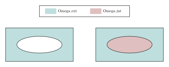
Fig. 41 g1 (on the left) and g2 (on the right)

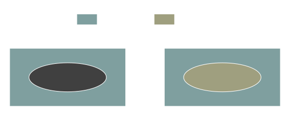
Fig. 42 g1 (on the left) and g2 (on the right)

This generates for g1 a rectangle with an elliptic hole, with only one surface domain “Omega_ext”. For g2, this generates a rectangle with 3 surface domains:

• “Omega_ext” will be the domain of the difference between the rectangle and the ellipse (the same as in g1)

• “Omega_int” will be the domain inside the ellipse

• “Omega” will be the union of “Omega_ext” and “Omega_int”

When using +, XLiFE++ checks if the rectangle is inside the ellipse and if the ellipse is inside the rectangle. It finds that the second check is true. If XLiFE++ is not able to determine the inclusion, it will warn you and consider that the inclusion does not exists.

When using -, XLiFE++ also checks the possible inclusions but considers this time that the “hole” (here the ellipse) is inside the “container” (here, the rectangle), whatever the results of the checks.

Tip

WHen using += or -= operators to define a composite geometry with a loop, you need to initiaize the composite geometry with the first component with the toComposite routine. g1 in previous examplecould have been defined as follows:

Rectangle r(_xmin=-3, _xmax=3, _ymin=-2, _ymax=2, _nnodes=Numbers(33,22), _domain_name="Omega_ext");
Ellipse e(_center=Point(0,0), _xlength=1, _ylength=0.5, _nnodes=11, _domain_name="Omega_int");
Geometry g1=toComposite(r);
g1-=e;

Please see Combining geometries for more details.

Geometries defined from their boundaries

Another possibility is to define geometries from their boundaries, thanks to routines surfaceFrom (for 2d geometries) and volumeFrom (for 3d geometries). The following example shows how to define a rounded rectangle:

Point a(-1.5,-4.), b(1.5,-4.), c(2.,-3.5), d(2.,3.5);
Point e(1.5,4.), f(-1.5,4.), g(-2.,3.5), h(-2.,-3.5);
Segment s1(_v1=a, _v2=b, _nnodes=21, _domain_name="AB");
CircArc c1(_center=Point(3.5,0.5), _v1=b, _v2=c, _nnodes=5, _domain_name="BC");
Segment s2(_v1=c, _v2=d, _nnodes=11, _domain_name="CD");
CircArc c2(_center=Point(3.5,1.5), _v1=d, _v2=e, _nnodes=5, _domain_name="DE");
Segment s3(_v1=e, _v2=f, _nnodes=21, _domain_name="EF");
CircArc c3(_center=Point(0.5,1.5), _v1=f, _v2=g, _nnodes=5, _domain_name="FG");
Segment s4(_v1=g, _v2=h, _nnodes=11, _domain_name="GH");
CircArc c4(_center=Point(0.5,0.5), _v1=h, _v2=a, _nnodes=5, _domain_name="HA");
Geometry roundedRect=surfaceFrom(s1+c1+s2+c2+s3+c3+s4+c4);

Fig. 43 roundedRect

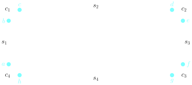
Fig. 44 roundedRect

Each component of the boundary of roundedRect will be a boundary domain: “AB”, “BC”, “CD”, “DE”, “EF”, “FG”, “GH”, and “HA”. There will be also a surface domain named “Omega”.

Caution

For 2d geometries, as in the current example, the different boundary geometries have to be defined with the same orientation.

Please see Definition of a geometry from its boundary for more details.

About inclusions

In the previous sections, you learn how to define geometries from their boundaries (loop geometries), and how to combine geometries. Of course, you can combine loop geometries and composite geometries. When at least a parallelepiped, an ellipsoid, a parallelogram or an ellipse in involved, XLiFE++ is always able to check inclusion. In other cases, it may fail. In this case, XLiFE++ warns you that it did not succeed in checking the inclusions, then you have the possibility to force inclusion (as for - operator) by using the unary + operator. Let’s see a more advanced example, where it is necessary:

Ellipse e1(_center=Point(0.,0.), _v1=Point(4,0.), _v2=Point(0.,5.), _nnodes=12, _domain_name="Omega1");
Point a(-1.5,-4.); Point b(1.5,-4.); Point c(2.,-3.5); Point d(2.,3.5);
Point e(1.5,4.); Point f(-1.5,4.); Point g(-2.,3.5); Point h(-2.,-3.5);
Segment s1(_v1=a, _v2=b, _nnodes=21, _domain_name="AB");
CircArc c1(_center=Point(3.5,0.5), _v1=b, _v2=c, _nnodes=5, _domain_name="BC");
Segment s2(_v1=c, _v2=d, _nnodes=11, _domain_name="CD");
CircArc c2(_center=Point(3.5,1.5), _v1=d, _v2=e, _nnodes=5, _domain_name="DE");
Segment s3(_v1=e, _v2=f, _nnodes=21, _domain_name="EF");
CircArc c3(_center=Point(0.5,1.5), _v1=f, _v2=g, _nnodes=5, _domain_name="FG");
Segment s4(_v1=g, _v2=h, _nnodes=11, _domain_name="GH");
CircArc c4(_center=Point(0.5,0.5), _v1=h, _v2=a, _nnodes=5, _domain_name="HA");
Geometry sf1=surfaceFrom(s1+c1+s2+c2+s3+c3+s4+c4,"Omega2");
Ellipse e2(_center=Point(1.,2.), _v1=Point(1.5,2.), _v2=Point(1.,3.), _nnodes=12, _domain_name="Omega3");
Ellipse e3(_center=Point(0.,0.), _v1=Point(0.5,0.), _v2=Point(0.,1.), _nnodes=12, _domain_name="Omega4");
Rectangle r2(_xmin=5., _xmax=6., _ymin=0., _ymax=1., _nnodes=6, _domain_name="Omega5");
Segment s5(_v1=Point(5.3,0.5), _v2=Point(5.7,0.5), _nnodes=5);
CircArc c5(_center=Point(5.5,0.5), _v1=Point(5.7,0.5), _v2=Point (5.5,0.7), _nnodes=5);
CircArc c6(_center=Point(5.5,0.5), _v1=Point (5.5,0.7), _v2=Point(5.3,0.5), _nnodes=5);
Geometry sf2=surfaceFrom(s5+c5+c6,"Omega6");
Geometry composite = e1+(sf1+(+(e2+e3)))+(r2-sf2);

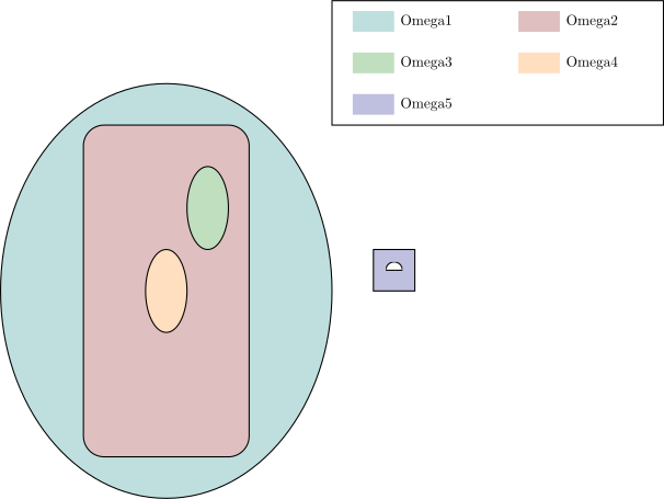
Fig. 45 composite

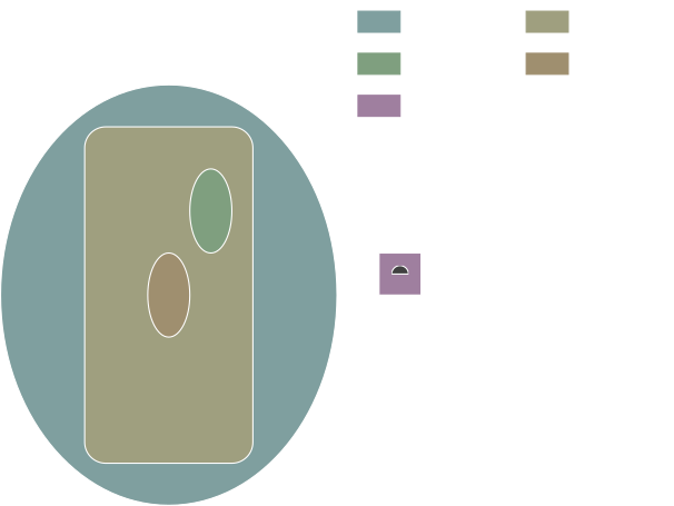
Fig. 46 composite

This generates a complex composite geometry with the following domains:

• “Omega1” will be the domain of the difference between the ellipse and the rounded rectangle

• “Omega2” will be the domain of the difference between the rounded rectangle and both small ellipses

• “Omega3” will be the domain inside the top right small ellipse

• “Omega4” will be the domain inside the bottom left small ellipse

• “Omega5” will be the domain of the difference between the rectangle and the half-disk

• “Omega” will be the union of “Omega1”, “Omega2”, “Omega3”, “Omega4”, “Omega5”

As far as detection of inclusions is concerned:

• As e2+e3 is a composite geometry and sf1 is a loop geometry, the unary + is required to ensure that both ellipses are considered as holes of the rounded rectangle, and the resulting composite geometry will be enclosed by parentheses;

• as e1 is an ellipse, the rounded rectangle sf1+(+(e2+e3)) will be confirmed inside;

• as e1 is an ellipse, r2-sf2 will be confirmed outside each other;

• as the configuration is not too tricky, r2-sf2 and sf1+(+(e2+e3)) will be confirmed outside each other.

Tip

When you define composite geometries with a lot of components, the default behavior is to check the inclusion for each pair of components. When you know where the holes will be, you can restrict the check to the appropriate container.

This is the reason why r2-sf2 is between parentheses. Is it useless to check if sf2 is inside the other components.

Transformations on geometries

Geometrical transformations on geometries work as on points. Then, if you want to apply a transformation and modify the input object, you can use one of the following functions:

• translate to apply a translation

• rotate2d to apply a 2D rotation

• rotate3d to apply a 3D rotation

• homothetize to apply a homothety

• pointReflect to apply a point reflection

• reflect2d to apply a 2D reflection

• reflect3d to apply a 3D reflection

For instance:

Segment s(_v1=Point(0.,0.,0.), _v2=Point(0.,0.,0.), _nnodes=10, _domain_name="S1");
s.translate(_direction={0.,0.,1.});

Please see Geometrical transformations for definition and use of transformations routines.

However, if you want now to create a new object by applying a transformation on a geometry, you should use one of the related external functions instead.

For instance:

Segment s(_v1=Point(0.,0.,0.), _v2=Point(0.,0.,0.), _nnodes=10, _domain_name="S1");
Segment s2=translate(s, _direction={0.,0.,1.});

Important

When transforming a geometry, domain names are changed. Indeed, the transformation adds a suffix “_prime”.

Important

Transforming a Geometry, applies also the transformation on the underlying bounding box.

Extrusion of geometries

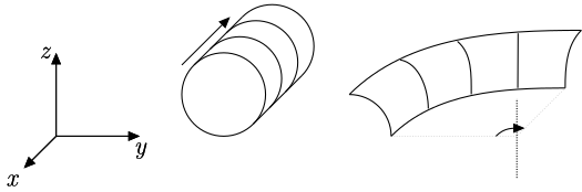
This is another way to define geometries : by extrusion of geometries of lesser dimension. Extruded geometries can be surfaces or volumes, defined by a geometry (the section of the extruded geometry) and a geometrical transformation. This feature can be used to generate meshes with the Gmsh interface with some restrictions about the transformation: only translations or rotations are authorized. There is also another parameter: the number of layers. Let’s see the following figures:

On the left, extrusion of a disk by a translation, with 3 layers. On the right, extrusion of a circular arc by rotation, with 4 layers

How to apply an extrusion ?

XLiFE++ offers 4 variants of the same function to define a Geometry by extrusion, enabling to give the domain name to the extruded geometry and to its sides. Sides numbering is as follows : first, the geometry used as section of the extrusion, second, the other section, and next the lateral surfaces generated by the extrusion.

Geometry extrude(const Geometry& g, const Transformation& t, Number layers);
Geometry extrude(const Geometry& g, const Transformation& t, Number layers, String domName);
Geometry extrude(const Geometry& g, const Transformation& t, Number layers, Strings sidenames);
Geometry extrude(const Geometry& g, const Transformation& t, Number layers, String domName, Strings sidenames);

The Geometry given to the extrude function can be:

• a canonical one (1D or 2D). Here, a CircArc:

  Point b(1.5,-4.,0.);
  Point c(2.,-3.5,0.);
  CircArc g(_center=Point(1.5,-3.5,0.), _v1=b, _v2=c, _nnodes=5, _domain_name="BC");
  Geometry e2d=extrude(g, Translation(0.,0.,4.), 5, "Omega");
  

  

  Fig. 47 Extrusion of a circular arc by translation, with 5 layers.

• A loop geometry (1D or 2D). Here, a rounded rectangle defines as in Definition of a geometry from its boundary:

  Point a(-1.5,-4.,0.); Point b(1.5,-4.,0.); Point c(2.,-3.5,0.); Point d(2.,3.5,0.);
  Point e(1.5,4.,0.); Point f(-1.5,4.,0.); Point g(-2.,3.5,0.); Point h(-2.,-3.5,0.);
  Segment s1(_v1=a, _v2=b, _nnodes=21, _domain_name="AB");
  CircArc c1(_center=Point(3.5,0.5,0.), _v1=b, _v2=c, _nnodes=5, _domain_name="BC");
  Segment s2(_v1=c, _v2=d, _nnodes=11,  _domain_name="CD");
  CircArc c2(_center=Point(3.5,1.5,0.), _v1=d, _v2=e, _nnodes=5,  _domain_name="DE");
  Segment s3(_v1=e, _v2=f, _nnodes=21,  _domain_name="EF");
  CircArc c3(_center=Point(0.5,1.5,0.), _v1=f, _v2=g, _nnodes=5,  _domain_name="FG");
  Segment s4(_v1=g, _v2=h, _nnodes=11,  _domain_name="GH");
  CircArc c4(_center=Point(0.5,0.5,0.), _v1=h, _v2=a, _nnodes=5,  _domain_name="HA");
  Geometry g=planeSurfaceFrom(s1+c1+s2+c2+s3+c3+s4+c4,"Omega");
  Geometry e3d=extrude(g, Translation(0.,0.,4.), 10, "Omega");
  

  

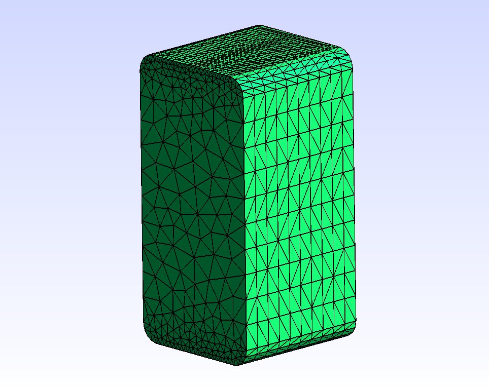
  Fig. 48 Extrusion of a rounded rectangle (loop geometry) by a rotation, with 10 layers.

• Every composite geometry composed exclusively of a geometry and its holes (1D or 2D). That is to say only operator- or operator-= is used to define the geometry:

  Ellipse e1(_center=Point(0.,0.,0.), _v1=Point(4,0.,0.), _v2=Point(0.,5.,0.), _nnodes=12, _domain_name="Omega1", _edge_names=Strings("Gamma_1","Gamma_2","Gamma_3","Gamma_4"));
  Ellipse e2(_center=Point(1.,2.,0.), _v1=Point(1.5,2.,0.), _v2=Point(1.,3.,0.), _nnodes=12, _domain_name="Omega3", _edge_names=Strings("Gamma_9","Gamma_10","Gamma_11","Gamma_12"));
  Geometry e3d2=extrude(e1-e2, Rotation3d(Point(5.,0.,0.), 0., 5., 0., pi_/2.), 10, "Omega", "Gamma");
  

  

  Fig. 49 Extrusion of an ellipse with an elliptical hole by rotation, with 10 layers.

How to define names of lateral domains of an extrusion ?

Instead of giving the same name to every lateral surface of an extrusion, it is possible to name each of them, but what about sides numbering ?

First example, let’s take the extrusion of a CircArc:

Point b(1.5,-4.,0.);
Point c(2.,-3.5,0.);
CircArc g(_center=Point(1.5,-3.5,0.), _v1=b1, _v2=c1, _nnodes=5, _domain_name="BC");
Geometry e2d=extrude(g, Translation(0.,0.,4.), 5, "Omega", Strings("Gamma1", "Gamma2"));

In Extrusion of geometries, point \(b\) is the front below left corner and point \(c\) is the front top right corner. As \(g\) is defined from \(b\) to \(c\), the first lateral side, corresponding to domain \(Gamma1\), will be the edge below. If \(g\) is defined from \(c\) to \(b\), \(Gamma1\) would have corresponded to the edge above.

Second example, let’s take the extrusion of an ellipse with an elliptical hole:

Ellipse e1(_center=Point(0.,0.,0.), _v1=Point(4,0.,0.), _v2=Point(0.,5.,0.), _nnodes=12, _domain_name="Omega1");
Ellipse e2(_center=Point(1.,2.,0.), _v1=Point(1.5,2.,0.), _v2=Point(1.,3.,0.), _nnodes=12, _domain_name="Omega3");
Geometry e3d3=extrude(e1-e2, Rotation3d(Point(5.,0.,0.), 0., 5., 0., pi_/2.), 10, "Omega", Strings("Gamma1", "Gamma2", "Gamma3", "Gamma4", "Gamma5", "Gamma6", "Gamma7", "Gamma8"));

This time lateral surfaces are ordered as follows:

• Lateral surfaces from the outer ellipse are ordered the same way as borders of the ellipse

• Lateral surfaces from the inner ellipse (and every hole in general) are ordered in the reverse order of borders of the ellipse

Warning

Contrary to Gmsh, extrusion of a geometry by rotation of angle greater than \(\pi\) is available, by splitting extrusion in 2 half extrusions when angle is not \(2\pi\) or in 4 quarter extrusions when angle is \(2\pi\). As a result, the number of lateral surfaces is multiplied by 2 or 4.

Example: definition of a conesphere

To define geometries based on cones, extrusions have to be used. It is the case for the conesphere:

Real rb=1., hc=3.;
Real hs=rb*rb/hc;
Real rs=sqrt(rb*rb + hs*hs);

Point origin(0.,0.,0.), apex(0.,0.,hc), p1(rb,0.,0.), p2(0.,0.,-hs-rs);

Segment s1(_v1=p1, _v2=apex, _hsteps=0.05);
Segment s2(_v1=apex, _v2=origin, _hsteps=0.05);
Segment s3(_v1=origin, _v2=p2, _hsteps=0.05);
CircArc c1(_center=Point(0.,0.,-hs), _v1=p2, _v2=p1, _hsteps=0.05);
Disk d1(_center=0.5*p1, _v1=0.5*p1+Point(0.2*rb,0.,0.), _v2=0.5*p1+Point(0.,0.,0.2*rb), _domain_name="Sigma", _hsteps=0.05);

Geometry base=planeSurfaceFrom(s2+s3+c1+s1, "Gamma");
Geometry g=extrude(base, Rotation3d(Point(0.,0.,0.), 0., 0., 1., 2.*pi_), "Omega1", Strings("Gamma1", "Gamma2", "Gamma3", "Gamma4", "Gamma5", "Gamma6", "Gamma7", "Gamma8"));

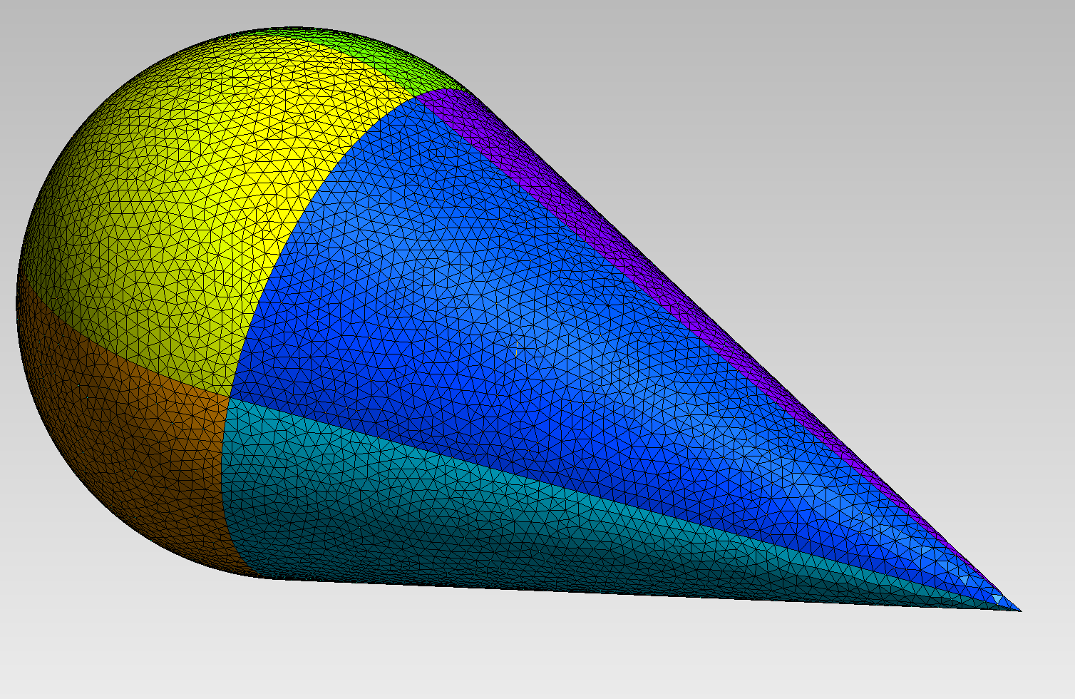
Fig. 50 Mesh of a conesphere.

OpenCASCADE extension

Open Cascade Technology (OCT) [1] is a third party open source library dedicated to 3D CAD data. It is a powerful library dealing with canonical geometries but providing complex geometrical operations (union, intersection, difference of geometries, fillet, chamfer, …). The standard geometry engine of XLiFE++ provides only union or difference in the case of one geometry included in another one (if detection is relatively easy). So to go further, XLiFE++ provides an interface to OCT. Obviously, OCT must be installed and activated in XLiFE++ (cmake option).

Footnotes

[1]

trademark @Open Cascade, https://www.opencascade.com/

Warning

OCT interface is still experimental. Use it with caution!

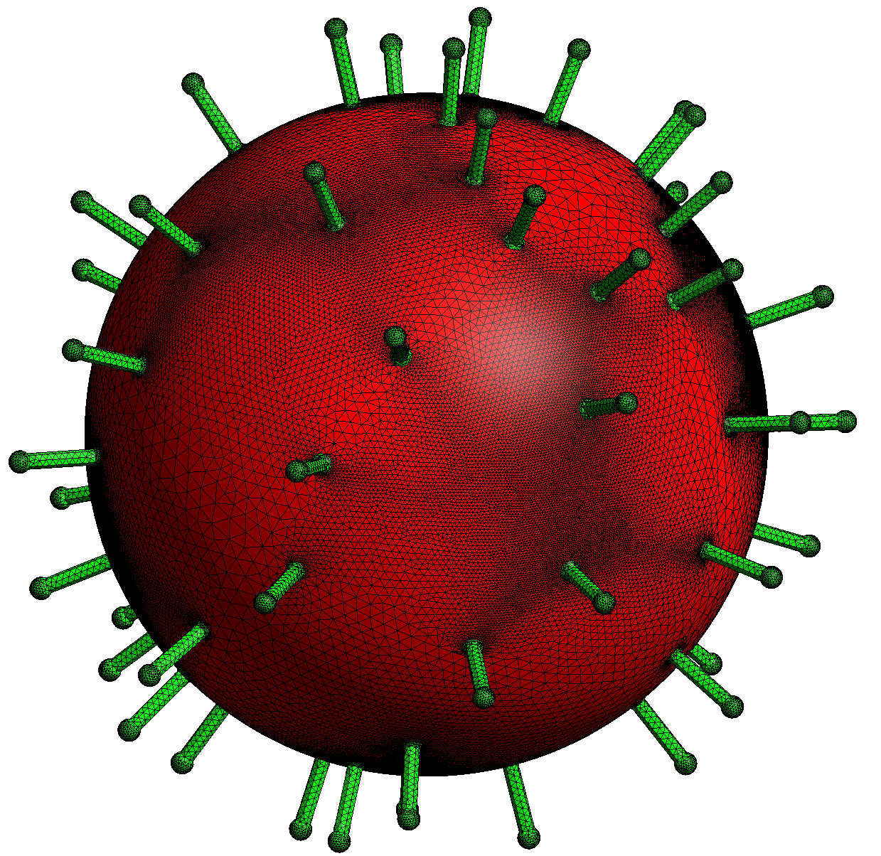
The next example, a light model of a virus, shows how powerful OCT is and how XLiFE++ can manage complex geometries. The main idea is to define a glycoprotein (a tentacle) by using a cone, a cylinder and a sphere, then to generate the set of glycoproteins by random rotations around a sphere, and then to fuse the whole set of elements:

Cone co(_center1=Point(0.,0.,0.), _v1=Point(1.,0.,0.), _v2=Point(0.,1.,0.), _apex=Point(0.,0.,1), _hsteps=0.3, _face_names="gamma");
Cylinder cy(_center1=Point(0.,0.,0.), _v1=Point(0.7,0.,0.), _v2=Point(0.,0.7,0.), _center2=Point(0.,0.,7.), _hsteps=1, _face_names="gamma");
Ball ba(_center=Point(0.,0.,7.), _radius=1., _hsteps=0.3, _face_names="gamma");
Geometry ant=cy+co+ba;
Real R=30., aR=0.999*R, d=0.2;
Ball bacor(_center=Point(0.,0.,0.), _radius=R, _hsteps=2, _face_names="sigma");
Geometry cor=toComposite(bacor);
for (Number i=0; i<8; i++)
{
  for (Number j=0; j<7; j++)
  {
    Real ir = i+d*(2*std::rand() * (1.0 / RAND_MAX)-1), jr= j+d*(2*std::rand() * (1.0 / RAND_MAX)-1);
    Real t=pi_*(ir/4-1), p=pi_/8*(jr-3);
    Transformation tf = Translation(_direction={aR*cos(t)*cos(p), aR*sin(t)*cos(p), aR*sin(p)}) *
                        Rotation3d(_center=Point(0.,0.,0.), _axis={0.,0.,1.}, _angle=t);
    tf *= Rotation3d(_center=Point(0.,0.,0.), _axis={0.,1.,0.}, _angle=pi_/2-p);
    cor+=transform(ant, tf);
  }
}

Available geometrical operations

operation	with OC extension	standard geometry engine
+	merge geometries (fusion)	union of disjoint or included geometries
-	difference of geometries (cut)	make a hole (included geometries)
^	intersection of geometries (common)	not available
%	not managed	force inclusion

Importing brep files

OCT extension provides a new interesting feature : loading a BREP file in a Geometry object:

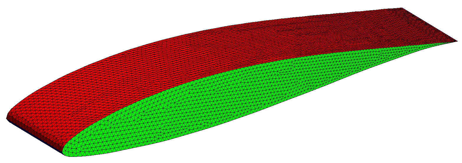
Geometry naca("NACA63-412.brep");
naca.setOCName(_solid, 1, "naca");
naca.setOCName(_face, 1, "extrados"); //extrados face
naca.setOCName(_face, 2, "intrados"); //intrados face
naca.setOCName(_face, Numbers(3,4), "lateral"); //lateral faces
naca.setOCHstep(Numbers(1,3), 0.2);
naca.setOCHstep(Numbers(2,4), 0.1);