Getting started

How does it work ?

The variational approach

Before learning in details what XLiFE++ is able to do, let us explain the basics with an example, the Neumann problem:

For a given function \(f(x,y)\), find a function \(u(x,y)\) satisfying:

(2)\[\begin{split}\begin{cases} -\Delta u(x,y) + u(x,y)=f(x,y) & \forall (x,y) \in \Omega \\ \dfrac{\partial u}{\partial n}(x,y)=0 & \forall (x,y) \in \partial\Omega \end{cases}\end{split}\]

To solve this problem by a finite element method, XLiFE++ is based on its variational formulation:

Find \(u\in H^1(\Omega)\) such that \(\forall v\in H^1(\Omega)\):

(3)\[\int_\Omega\nabla u.\nabla v\,dx\,dy +\int_\Omega u\,v\,dx\,dy=\int_\Omega f\,v\,dx\,dy.\]

All the mathematical objects involved in the variational formulation are handled in XLiFE++ : domain, approximation space, differential operators, …

Tutorial: Neumann problem

The following program solves the Neumann problem with \(f(x,y)=\cos{\pi x} \cos{\pi y}\) and \(\Omega\) is the unit square.

#include "xlife++.h"
using namespace xlifepp;

Real cosxcosy(const Point& P, Parameters& pa = defaultParameters)
{
  Real x=P(1), y=P(2);
  return cos(pi_ * x) * cos(pi_ * y);
}

int main(int argc, char** argv)
{
  init(_lang=fr); // mandatory initialization of xlifepp
  SquareGeo sq(_origin=Point(0.,0.), _length=1, _nnodes=11);
  Mesh mesh2d(sq, _generator=structured);
  Domain omega = mesh2d.domain("Omega");
  Space Vk(_domain=omega, _interpolation=P1, _name="Vk", _optimizeNumbering);
  Unknown u(Vk, _name="u");
  TestFunction v(u, _name="v");
  BilinearForm auv = intg(omega, grad(u) | grad(v)) + intg(omega, u * v);
  LinearForm fv=intg(omega, cosxcosy * v);
  TermMatrix A(auv, _name="a(u,v)");
  TermVector B(fv, _name="f(v)");
  TermVector X0(u, omega, 1., _name="X0");
  TermVector U = cgSolve(A, B, X0, _name="U");
  saveToFile("U.vtu", U);
  return 0;
}

Please notice how close to Mathematics XLiFE++ user language is.

Step-by-step explanations

This first example shows how XLiFE++ executes all the usual steps required by the Finite Element Method. Let us walk through them one by one.

• Every program using XLiFE++ has to include the main header file:

  #include "xlife++.h"
  

  This “super” header xlife++.h loads some global variables and functions:

  • Mathematical constants (pi_, i_, …);

  • Global functions managing locally the verbosity, the number of threads, …;

  • Timers;

  • …

  See XLiFE++ global parameters for more details about them.

  Warning

  If users have additional source files using XLiFE++ elements, they cannot include the “super” header file xlife++.h because of these global variables and functions. This is the reason why in these additional source files, you will include the “super” header file xlife++-libs.h instead.

• Every object or function of XLiFE++ is defined inside a namespace called xlifepp. So, the following line prevents the user from specifying each time he/she uses an object or a function of XLiFE++:

  using namespace xlifepp;
  

• Every program using XLiFE++ begins by a call to the init() function, taking up to 4 key/value arguments but only 2 are relevant for users:

  _verbose

  integer to set the verbose level. Default value is 1.

  _lang

  enum to set the language for print and log messages. Possible values are en for English, fr for French, de for German, or es for Spanish. Default value is en.

  Furthermore, the init() function loads functionalities linked to the trace of where such messages come from. If this function is not called, XLiFE++ cannot work !!!

    init(_lang=fr); // mandatory initialization of xlifepp
  

  See Global variables and parameters to learn how to define command line options or options files specific to your program and how to use them.

  You can define your own command-line options to manage parameters and avoid useless compilation steps. See Management of custom options (Options class) for more details.

• The mesh will be generated on the unit square geometry with 11 nodes per edge. Arguments of a geometry are given with a key/value system. _origin is the bottom left front vertex of SquareGeo. Next, we can specify the mesh element type (here triangle, the default value for 2d geometries), the mesh element order (here 1, the default), the mesh tool given by the key generator (here structured). The main mesh tools are structured for simple geometries (rectangle, cube, …) and gmsh for general geometries. See Generating a mesh from a geometry for more examples of mesh definitions.

    SquareGeo sq(_origin=Point(0.,0.), _length=1, _nnodes=11);
    Mesh mesh2d(sq, _generator=structured);
  

• The main domain, named “Omega” in the mesh, is defined in a specific variable that will be used in the following:

    Domain omega = mesh2d.domain("Omega");
  

• A finite element space is generally a space of polynomial functions on elements, triangles here only. Here sp is defined as the space of continuous functions which are affine on each triangle \(T_k\) of the domain \(\Omega\), usually named \(V_h\). The dimension of such a space is finite, so we can define a basis

  \[sp(\Omega,P1)=\left\{ w(x, y) \mathrm{\;such\;that\;} \exists (w_1, \ldots, w_N) \in \mathbb{R}^N, w(x, y) = \sum_{i=1}^N w_k \varphi_k(x, y)\right\},\]

  where \(N\) is the space dimension, i.e. the number of nodes (the number of vertices here).

    Space Vk(_domain=omega, _interpolation=P1, _name="Vk", _optimizeNumbering);
  

  Currently, XLiFE++ implements the following elements: \(P_k\) on segment, triangle and tetrahedron, \(Q^k\) on quadrangle and hexahedron, \(O_k\) on prism and pyramid (see Generating a mesh from a geometry for more details).

• The unknown \(u\) here is an approximation of the solution of the problem. \(v\) is declared as test function. This comes from the variational formulation of (2): multiplying both sides of equation and integrating over \(\Omega\), we obtain:

  \[-\int_{\Omega} v \Delta u \;dx dy +\int_{\Omega} v u\; dx dy = \int_{\Omega} v f \;dx dy\]

  Then, using Green’s formula, the problem is converted into finding \(u\) such that:

  (4)\[a(u, v) = \int_{\Omega} \nabla u \cdot \nabla v \;dx dy + \int_{\Omega} u v \;dx dy = \int_{\Omega} f v \;dx dy = l(v)\]

  The 4 next lines in the program declare \(u\) and \(v\) and define the forms \(a\) and \(l\).

    Unknown u(Vk, _name="u");
    TestFunction v(u, _name="v");
    BilinearForm auv = intg(omega, grad(u) | grad(v)) + intg(omega, u * v);
    LinearForm fv=intg(omega, cosxcosy * v);
  

  Please notice that:

  • The test function is defined from the unknown. The reason is that the test function is dual to the unknown. Through the unknown, \(v\) is also defined on the same space.

  • The right-hand side needs the definition of the function \(f\). Such function can be defined as a classical C++ function, but with a particular prototype.

    Real cosxcosy(const Point& P, Parameters& pa = defaultParameters)
    {
      Real x=P(1), y=P(2);
      return cos(pi_ * x) * cos(pi_ * y);
    }
    

    In this example, \(f\) (i.e. cosxcosy) is a scalar function. So it takes 2 arguments : the first one is a Point, containing coordinates \(x\) and \(y\). The second one is optional and contains parameters to use inside the function. Here, the Parameters object is not used. At last, as a scalar function, it returns a Real, but it could be a Complex or a real/complex vector (Reals, Complexes).

• The previous definitions are a description of the variational form. Now, we have to build the matrix and the right-hand side vector which are the algebraic representations of the linear forms in the finite element space.

  \[A_{i,j}=a(\varphi_j,\varphi_j) \mathrm{\;and\;} B_i=\int_{\Omega}f\,\varphi_i\]

  This is done by the following lines:

    TermMatrix A(auv, _name="a(u,v)");
    TermVector B(fv, _name="f(v)");
  

• Once matrix and vector are computed, you can now choose the solver you want. Here, a conjugate gradient solver is used with an initial guess vector equal to the constant vector 1.

    TermVector X0(u, omega, 1., _name="X0");
    TermVector U = cgSolve(A, B, X0, _name="U");
  

  XLiFE++ offers you a various choice of direct or iterative solvers:

  • LU, LDU, LL^t, LDL^t, LDL^* factorizations or Gauss solver

  • BICG, BiCGStab, CG, CGS, GMRES, QMR, SOR, SSOR, solvers

  • internal eigen solver

  • wrappers to external packages such as UmfPack, Arpack

  See Algebraic representation and Solvers for more details.

• To save the solution, XLiFE++ provides an export to Paraview format file (vtu).

    saveToFile("U.vtu", U);
  

  It is also possible to export to other formats, such as ones destined to Gmsh or Matlab for instance.

• Do not forget to end properly your program. A C++ “main” function always ends with the foloowing line, saying that everything is fine.

    return 0;
  

Let’s now see how to compile such programs.

Compile a program using XLiFE++

The graphical way

macOS

This way is possible to make easier the manual way and more pleasant than the command-line way. On the website, you have a GUI application called xlifepp-qt for macOS, (Windows and Unix/Linux will come soon). You can define a shortcut on it wherever you want.

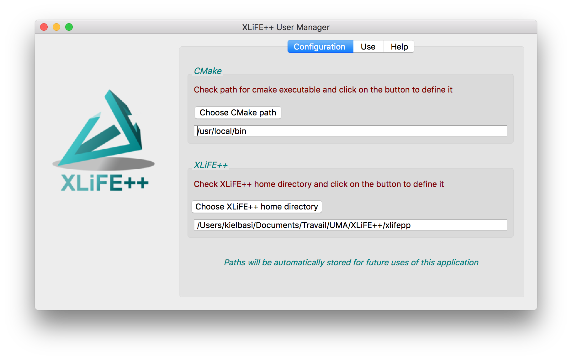
Fig. 36 The Configuration tab of xlifepp-qt application

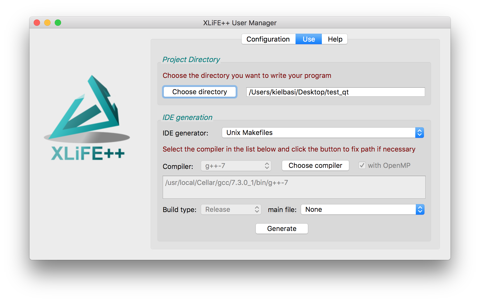
Fig. 37 The Use tab of xlifepp-qt application

This application is a graphical user interface to the first 3 steps of the manual way.

Windows

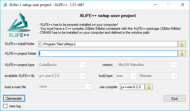
1. You run the generator xlifepp_new_project.exe located in the bin subdirectory of the XLiFE++ install directory. The XLiFE++ folder should be correct but you can fix it if necessary.

   

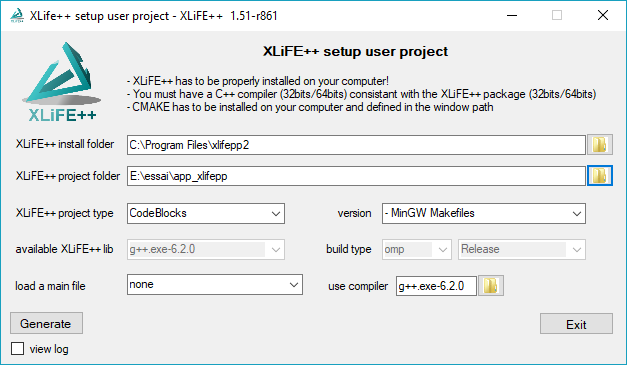
2. You select the folder in which you will write your program using XLiFE++. If it already exists, the generator asks you to clean it or not. This window gives some information about XLiFE++: the compiler used to generate it, if the library supports omp and the debug/release status. You should use a compatible compiler with this library. If the default C++ compiler found on your computer is not compatible, you can select another one by clicking on the use compiler folder button.

   

3. Select the type of your project. For the moment only CodeBlocks - MinGW and Makefile are working but CodeBlocks is highly recommended! Select a main file from the proposed list. This main file will be copied in your application folder. Be careful, if you choose “none”, no main file will be copied and the generator will fail if there is no main file in your application folder. This option is only useful if you want to keep an existing main file in your application folder! Click on the Generate button and wait:

   

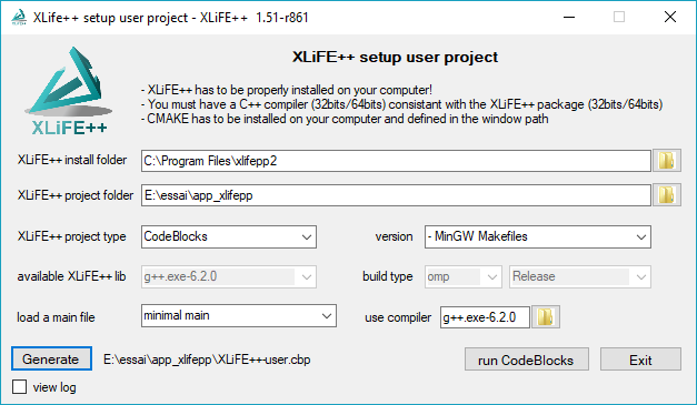
4. When everything is complete, you can either exit the tool or run the program that opens the generated project (CodeBlocks in the example) by clicking on the run button.

The command-line way

This way is possible to make easier the manual way. In the bin directory of XLiFE++, you have shell script called xlifepp.sh for macOS and Linux, and a batch script called xlifepp.bat. You can define a shortcut on it wherever you want.

Here follows an example showing how to use XLiFE++ with these command-line tools.

We can create an executable file. To do that, we choose to create a test directory and to compile one of the examples present in this documentation:

$ mkdir /tmp/test
$ cd /tmp/test
$ ~/xlifepp/bin/xlifepp.sh
*********************************
*           xlifepp             *
*********************************
Project directory (default is current directory):

/tmp/test exists
The following generators are available on this platform:
1 -> Unix Makefiles
2 -> Ninja
3 -> Xcode
4 -> CodeBlocks - Ninja
5 -> CodeBlocks - Unix Makefiles
6 -> CodeLite - Ninja
7 -> CodeLite - Unix Makefiles
8 -> Sublime Text 2 - Ninja
9 -> Sublime Text 2 - Unix Makefiles
10 -> Kate - Ninja
11 -> Kate - Unix Makefiles
12 -> Eclipse CDT4 - Ninja
13 -> Eclipse CDT4 - Unix Makefiles
14 -> KDevelop3
15 -> KDevelop3 - Unix Makefiles
Your choice (default is 1): 1
The following compilers are available:
1 -> clang++-4.2.1
The following main files are available:
1 -> main.cpp
2 -> elasticity2dP1.cpp
3 -> helmholtz2d-Dirichlet_single_layer.cpp
4 -> helmholtz2dP1-DtN_scalar.cpp
5 -> helmholtz2dP1-cg.cpp
6 -> helmholtz2d_FEM_BEM.cpp
7 -> helmholtz2d_FE_IR.cpp
8 -> helmholtz3d-Dirichlet_single_layer.cpp
9 -> laplace1dGL60-eigen.cpp
10 -> laplace1dP1.cpp
11 -> laplace1dP10Robin.cpp
12 -> laplace2dP0_RT1.cpp
13 -> laplace2dP1-average.cpp
14 -> laplace2dP1-dirichlet.cpp
15 -> laplace2dP1-periodic.cpp
16 -> laplace2dP1_Neumann.cpp
17 -> laplace2dP2-eigen.cpp
18 -> laplace2dP2-transmission.cpp
19 -> maxwell2dN1.cpp
20 -> maxwell3D_EFIE.cpp
21 -> wave_2d_leap-frog.cpp
Your choice (default is 1): 14
Copying laplace2dP1-dirichlet.cpp
Cleaning CMake build files
You can use:
1 -> sequential
The following build types are available
1 -> Release
Copying CMakeLists.txt
-- The CXX compiler identification is AppleClang 9.1.0.9020039
-- Check for working CXX compiler: /usr/bin/clang++
-- Check for working CXX compiler: /usr/bin/clang++ -- works
-- Detecting CXX compiler ABI info
-- Detecting CXX compiler ABI info - done
-- Detecting CXX compile features
-- Detecting CXX compile features - done
-- OpenMP is not used
-- XLiFE++ was compiled with clang++-4.2.1
-- XLiFE++ was compiled without OpenMP
-- XLiFE++ was compiled in Release mode
-- XLiFE++ libraries found !
-- Arpack is used
-- Umfpack is used
-- LAPACK is used
-- BLAS is used
-- AMOS is used
-- Magma is not used
-- Metis is not used
-- MPI is not used
-- Configuring done
-- Generating done
-- Build files have been written to: /tmp/test
$ make
Scanning dependencies of target checklock
[  0%] Built target checklock
Scanning dependencies of target exec-x86_64-darwin-clang++-4.2.1-Release
[ 50%] Building CXX object CMakeFiles/exec-x86_64-darwin-clang++-4.2.1-Release.dir/laplace2dP1-
dirichlet.cpp.o
[100%] Linking CXX executable exec-x86_64-darwin-clang++-4.2.1-Release
[100%] Built target exec-x86_64-darwin-clang++-4.2.1-Release
$ ./exec-x86_64-darwin-clang++-4.2.1-Release
__  __  __ _   ___  __
\ \/ / / /(_) / __\/__\_     _
 \  / / / | |/ _\ /_\_| |_ _| |_
 /  \/ /__| / /  //_|_   _|_   _|
/_/\_\____/_\/   \__/ |_|   |_|

XLiFE++ v2.0.1-r79 (2018-07-20)
running on july 25, 2018 at 16h08 on Darwin-i386 (MacBook-Pro)

computing FE term intg_Omega grad(u) | grad(v), using 1 threads :  done
reducing FE term A using pseudo reduction method
TermMatrix A computed, size 400 X 400 : SuTermMatrix A_u_v : block (v, u) -> matrix 400 X 400
of real scalar in symmetric_compressed sparse (csr,csc) (1521 coefficients)

solving linear system A * X = B (size 400) using umfpack
$ ls
CMakeCache.txt     cmake_install.cmake
CMakeFiles         exec-x86_64-darwin-clang++-4.2.1-Release
CMakeLists.txt     laplace2dP1-dirichlet.cpp
Makefile           log.txt
U_LD_Omega.vtu     print.txt

The result file U_LD_Omega.vtu can then be displayed using Paraview.

Here is the list of general options of the script:

-b, --build	to copy cmake files and eventually sample of main file and run cmake on it to prepare your so-called project directory. This is the default
-g, --generate	to generate the project. Used with –build option. This is the default.
-h, -help, --help	to print the help
-i, --interactive	to run xlifepp in interactive mode. Used with –build option. This is the default
-noi, --non-interactive	to run xlifepp in non-interactive mode. Used with –build option
--no-generate, -nog	to prevent generation of your project. You will do it by yourself.
-v, --version	to print version number of XLiFE++ and its date
--verbose-level <value>, -vl <value>	to set the verbose level. Default value is 1

See also

Here is the list of specific options when in non-interactive mode:

--build-type <value>, -bt <value>	to set cmake build type (Debug, Release, …).
--cxx-compiler <value>, -cxx <value>	to set the C++ compiler to use.
--directory <dir>, -d <dir>	to set the directory where you want to build your project
--generator-name <name>, -gn <name>	to set the cmake generator.
-f <filename>, --main-file <filename>	to copy <filename> as a main file for the user project.
-nof, --no-main-file	not to copy the sample main.cpp file. This is the default.
--info-dir, -id	to set the directory where the info.txt file is
--with-omp, -omp	to activate OpenMP mode
--without-omp, -nomp	to deactivate OpenMP mode

The manual way

This way supposes that you know where XLiFE++ is installed.

1. You create your working directory,

2. You copy the main.cpp file into your working directory,

3. You copy the CMakeLists.txt file from the build directory (the directory in which you ran installation process) into your working directory,

4. You run Cmake on the CMakelists.txt file to get your makefile or files for your IDE project (Eclipse, XCode, CodeBlocks, Visual C++, …),

5. You can now edit the main.cpp file to write your program and enjoy compilation with XLiFE++.