Algebraic representation#

From the previous chapter (Problem definition), a discrete variational formulation has been defined:

\[\begin{split}\DeclareMathOperator{\spanop}{span} & \mathrm{Find\;} u \in V_h = \spanop (w_j)_{j=1,n}, \mathrm{\;such\;that\;} \forall v \in W_h = \spanop (\tau_j)_{j=1,m}, \\ & a(u,v) = l(v)\end{split}\]

Algebraic representation of the discrete formulation consists in going to a representation in terms of matrices and vectors. It leads generally to the solving of a linear system or the computation of eigenvalues and eigenvectors.

First, we can define vectors \(U\) and \(L\) as follows:

\[U=(u_j)_{j=1,n},\ L=\left(l(\tau_i)\right)_{i=1,m}\]

Next, by choosing \(v=\tau_i\), we can define matrix \(\mathbb{A}\) as follows:

\[\mathbb{A}=\left(a(w_j, \tau_i)\right)_{i=1,m,j=1,n}\]

At last, the discrete variational formulation gives the following linear system:

\[\mathbb{A} U = L\]

XLiFE++ provides two fundamental classes:

TermVector handles vectors related to a discrete approximation space (linear form, unknowns or test functions, DOF numbering, …)
TermMatrix handles matrices related to a discrete approximation space (bilinear form, unknowns and test functions, DOF numbering, …)

In the following, we will take a look at the standard operations about both classes. To go further, please go to the Algebraic representation reference.

Important

The computation algorithms find the minimal representation of vectors/matrices. It means that the size of vector/matrix is equal to the number of unknown/test function’s DOFs (DOFs = degrees of freedom) involved in the computation. For instance, a mass matrix on a boundary involves only DOFs supported by the boundary.

The value type (real or complex) is automatically managed by TermMatrix and TermVector classes.

Tip

When the result of a linear combination of terms involves complex values, the resulting term will be set to real if the imaginary part is null.

Sometimes, in an advanced usage, it may be useful to convert a real term to a complex one or access to real part or imaginary part of a complex term.

For this purpose, XLiFE++ offers complex, real, imag and abs routines.

Representation from forms#

TermMatrix and TermVector can be respectively defined from BilinearForm and LinearForm:

BilinearForm auv=intg(omega, grad(u)|grad(v));
TermMatrix A(auv, _name="A"); // the stiffness matrix
LinearForm lv=intg(omega, f*v);
TermVector L(lv, _name="L");

Caution

The _name is mandatory. Even if it is advised to set it for print purpose, but the name will also be used when saving such objects to a file.

About multiple unknowns terms#

Both classes support either single unknown or multiple unknowns representation. Multiple unknowns vector or matrix are represented by single unknown blocks:

\[\begin{split}\mathbb{A} = \begin{pmatrix} \mathbb{A}_{v_1,u_1} & \mathbb{A}_{v_1,u_2} & \cdots & \mathbb{A}_{v_1,u_N} \\ \mathbb{A}_{v_2,u_1} & \mathbb{A}_{v_2,u_2} & \cdots & \mathbb{A}_{v_2,u_N} \\ \vdots & \vdots & \cdots & \vdots \\ \mathbb{A}_{v_M,u_1} & \mathbb{A}_{v_M,u_2} & \cdots & \mathbb{A}_{v_M,u_N} \\ \end{pmatrix}, \qquad L=\begin{pmatrix} L_{v_1} \\ \vdots \\ L_{v_M} \\ \end{pmatrix}\end{split}\]

where \(u_1, \ldots u_N\) stands for unknowns and \(v_1, \ldots v_M\) stands for test functions, \(v_i\) being the test function associated to unknown \(u_i\).

Important

Unknowns correspond to matrix columns and test functions to matrix rows!

In case of a multiple unknown TermMatrix or TermVector, an unknown block may be extracted as follows:

Space V(_domain=omega, _interpolation=P1, _name="V");
Unknown u1(V, _name="u1"), u2(V, _name="u2");
TestFunction v1(u1, _name="v1"), v2(u2, _name="v2");
BilinearForm auv=intg(omega1, grad(u1)|grad(v1))+intg(omega2, grad(u2)|grad(v2));
TermMatrix A(auv, _name="A"); // multiple unknowns TermMatrix
LinearForm lv=intg(omega1, f1*v1)+intg(omega2, f2*v2);
TermVector L(lv, _name="L"); // multiple unknowns TermVector
TermMatrix A11=A(u1,v1); // extract (u1, v1) part, single unknown TermMatrix
TermVector L1=L(v1); // extract (v1) part, single unknown TermVector

The returned TermMatrix or TermVector is a copy of the extracted block.

Delaying computation#

When defined, TermVector and TermMatrix are automatically computed, except if the option _notCompute is set in definition of TermMatrix or TermVector.

To perform the real computation, the compute routine has to be called explicitly.

...
BilinearForm auv=intg(omega,grad(u)|grad(v));
TermMatrix A(auv, _notCompute, _name="A");
...
compute(A);

Definition from interpolated values#

Define nodal values of an analytical kernel#

A scalar/vector real/complex nodal value TermMatrix can be constructed form a two variables C++ function (i.e. a kernel \(K\)):

\[\mathbb{G}_{ij}=K(M_i,M_j)\quad M_i,\ M_j\text{ nodes of domains } \Sigma,\ \Gamma.\]

Here is an example:

Kernel K = Helmholtz3dKernel(...);

...
Domain sigma=..., gamma=...;
Unknown us(...), ug(...);
...
TermMatrix G(ug, gamma, us, sigma, K, _name="G");
TermMatrix dnG(ug, gamma, us, sigma, grad_y(K)|_ny, _name="dnG");

Hint

This construction works also with an operator on a kernel.

Define interpolated values of an analytical function#

Interpolation \(\Pi\) of a function \(f\) on shape functions \((w_i)\) is defined as follows:

\[\Pi : f \mapsto \Pi (f) = \sum_{i=1}^N d_i(f) w_i\]

\((d_i)_{i=1,N}\) are the generalized degrees of freedom (generalized means viewed as distributions) related to shape functions \((w_i)_{i=1,N}\).

For Lagrange finite elements, this results in:

\[d_i=\delta_{M_i}\ \rightarrow d_i(f)=f(M_i)\]

where \((M_i)_{i=1,N}\) are the Lagrange nodes. In this case, interpolated values are named “nodal values”.

Important

In the following, it will be explained how to build the interpolated values of a function, as defined above. To non Lagrange DOFs (not nodal), some coordinates are virtually associated to, so the “nodal interpolation” may be enforced by using the key _nodal

Define interpolated values of C++ functions#

A scalar/vector real/complex interpolated value TermVector can be defined from a C++ function given by users. Here is an example:

Real sinxcosy(const Point& p, Parameters& pa=defaultParameters)
{ Real x=p.x(), y=p.y(); return sin(x)*cos(y); }
...
Domain omega=...;
Unknown u(...);
TermVector tv(u, omega, sinxcosy);

See Functions and kernels for more details on how to define such functions and manipulating parameters through the Parameters object.

For Morley elements, degrees of freedom involve first order derivatives, say \((\partial_x f, \partial_y f)\). For Argyris elements, they involve second order derivatives, say \((\partial_{xx} f, \partial_{yy} f, \partial_{xy} f)\). This is the reason why, in order to compute interpolated values of an analytical function when using these finite elements, the analytical function but also its first order derivatives and / or second order derivatives must be given:

Real fx(const Point& P, Parameters& pa = defaultParameters)
{
  return P(1);
}
Vector<Real> gx(const Point& P, Parameters& pa = defaultParameters)
{
  Vector<Real> g(2, 0.);
  g(1)=1.;
  return g;
}
Vector<Real> g2x(const Point& P, Parameters& pa = defaultParameters)
{
  return Vector<Real>(3, 0.);
}
...
TermVector vx(u, omega, Function(fx), Function(gx)); //order 0/1 DOFs involved
TermVector wx(u, omega, Function(fx), Function(gx), Function(g2x)); // order 0/1/2 DOFs involved

It is also working for vector unknowns; in that case derivatives must be given as a unique vector collecting all the derivatives for each component \((\partial_{x} f_1, \partial_{y} f_1, \partial_{x} f_2, \partial_{y} f_2, \cdots)\).

Define nodal values of a symbolic function#

For classical functions (trigonometrical functions, hyperbolic functions, exponential functions, …), there is an easier way to define nodal values: with symbolic functions. Let’s see the previous example rewritten with a symbolic function:

Domain omega=...;
Unknown u(...);
TermVector tv(u, omega, sin(x_1)*cos(x_2));

A symbolic function, handled by the SymbolicFunction class, can use the cartesian coordinates (x_1, x_2, x_3) or the spherical coordinates (r_ theta_ phi_), and can be linear combination of elementary functions.

As for analytical functions, a TermVector can be defined from a symbolic function on TermVector (up to 4). The purpose here is to build a TermVector by a symbolic function applied directly on TermVector values. This supposes that all considered TermVector are defined on the same approximation space but with possible different unknowns.

Warning

This works only for single unknown TermVector defined on the same approximation space (but possibly on different unknowns).

Combine nodal values#

In a same way, it is possible to combine values of 2 TermVector using a C++ function taking up to 2 values (real or complex):

Real f(const Real& r1, const Real& r2)
{ ... }
...
Domain omega=...;
TermVector tv1(...), tv2(...);
TermVector tv(tv1, tv2, f, _name="F"); // tv=f(tv1, tv2)

Warning

This works only for single unknown TermVector defined on the same unknown.

Algebraic operations#

You can:

compute linear combinations (*, *=, /, /= with scalars, +, +=, -, -=) of TermMatrix or TermVector objects.

Important

In order to be more efficient, the linear combination of terms is delayed up to the assign (=) operation or a constructor operation. It means that some expression may not be evaluated and produce warning/error message related to LcTerm class.
multiply (* and *= operators) a TermMatrix object by a TermVector object, or by another TermMatrix object.

Hint

When combining more than two terms, especially for TermMatrix, it is better to write the summation in one step rather than in several steps.

Caution

The product between two TermMatrix is always generated in dense format.
compute the scalar product / hermitian product of 2 TermVector objects by using the | operator, that always returns a complex value.

Hint

The specific routines are innerProduct and hermitianProduct. To compute an inner product between a real TermVector and a complex TermVector, use the routine dotRC.
compute norms: - The \(l^2\) norm (Frobenius norm \(\sqrt{\sum|A_{ij}|^2}\)) of a TermMatrix with the routine normL2 - The \(l^\infty\) norm (\(\max_{i,j}|A_{i,j}|\) or \(\max_i|U_i|\)) of a TermMatrix or a TermVector with the routine norminfty - The math:l^1 norm (Manhattan norm \(\sum_i |U_i|\)) of a TermVector with the routine norm1 - The quadratic norm (\(\sqrt {\sum_i |U_i|^2}\)) of a TermVector with the routine norm2

Deal with essential conditions#

As previously mentioned, essential conditions are attached directly to TermMatrix. They must be specified when constructing a TermMatrix from a bilinear form:

BilinearForm auv=intg(omega, grad(u)|grad(v));
EssentialConditions ecs= (u|sigmaM = 1) & (u|sigmaP = 1);
TermMatrix A(auv, ecs, _name="A");

Hint

Essential conditions are never attached to a TermVector! When solving a system involving essential conditions, the TermVector representing the right-hand side of the system is automatically corrected to take into account essential conditions effects.

In few words, the process to take into account essential conditions is the following:

the essential conditions are transformed in a constraints’ system \(\mathbb{C}U=D\) where \(\mathbb{C}\) is a \(p\times n\) rectangular matrix (\(n\) the dimension of \(U\), \(p < n\))
the constraints’ system is then reduced to an upper triangular system using a QR algorithm : \(\mathbb{C}=[\mathbb{E}\ \mathbb{R}]\) with \(\mathbb{E}\) a \(q\times q\) invertible matrix (\(q\le p\)) and \(\mathbb{R}\) an upper triangular \(q\times n\) matrix
the constraints’ system, now reading \(U_e=\mathbb{E}^{-1}D-\mathbb{E}^{-1}\mathbb{R}U_r\), variables \(U_e\) may be substituted in terms of \(U_r\) variables to change the matrix and may be the right-hand side.

Note

The QR factorization process can detect redundant or conflicting constraints; in any case only one constraint is kept and a warning message is raised. It is the responsibility of the user to check if the result is correct when such situation arises.

The QR process stops when the pivot coefficient is below a tolerance factor (by default \(100\times \varepsilon_{mach}\approx 2.10^{-14}\) in double precision). If the tolerance factor is too low, due to rounding errors, some quasi-redundant conditions are not reduced, leading to quasi-ill-posed linear system. To overcome this problem, the tolerance factor may be increased:

EssentialConditions ecs = (ncross(ud)-ncross(ug)|Sigma=0);
ecs.redundancyTolerance(1.E-10);

Manage reduction methods#

Essential conditions, corresponding to an elimination of some DOFs and a reduction of the matrix and may be of right hand side vector. There are several ways to deal with this reduction:

pseudo-elimination, changing some matrix coefficients (row or column index corresponding to eliminated DOFs) without changing the size of the system but may be the storage (default).
real elimination, eliminating row and column corresponding to the eliminated DOFs, decreasing the size of the system and changing the storage as a consequence.
penalization, adding to the matrix, the matrix constraints affected with a large coefficient, may be changing the storage and having a significant impact on matrix conditioning.
dualization, using a Lagrange multiplier related to the constraints’ system, thus increasing the size of the system by adding matrix blocks.

The method is chosen with the _reduction key and a ReductionMethod object (_pseudoReduction, _realReduction, _penalizationReduction or _dualReduction). All of them are available for any set of essential conditions, with the following restrictions: the real elimination is not yet available with a matrix right-hand side, nor for a multiple unknowns matrix with constraints on a part of its unknowns; the penalization and the dualization do not handle different constraints on unknowns and test functions. The dualization adds, for each set of constraints, a Lagrange multiplier (a new unknown) and the matrix blocks \(\mathbb{C}^*\) and \(\mathbb{C}\); the resulting saddle point system is symmetric (if the matrix is) but indefinite, so use a LU factorization (or umfpack) or the GMRES solver. For eigenvalue problems, only the pseudo-reduction is relevant (see below).

If necessary, it is possible to change the diagonal coefficient (by default 1) of the pseudo eliminated block matrix by invoking the ReductionMethod object:

BilinearForm auv=intg(omega, grad(u)|grad(v));
EssentialConditions ecs= (u|sigmaM = 0);
TermMatrix A(auv, ecs, _reduction=ReductionMethod(_pseudoReduction, 10.), _name="A");

The penalization method adds \(\alpha\) to the diagonal coefficients related to DOFs where the Dirichlet conditions act. To use the penalization method, change the method in the ReductionMethod object:

BilinearForm auv=intg(omega, grad(u)|grad(v));
EssentialConditions ecs= (u|sigmaM = 0);
TermMatrix A(auv, ecs, _reduction=ReductionMethod(_penalizationReduction,10000.), _name="A");

Pseudo-reduction and eigenvalue problems#

When dealing with eigenvalue problems be very cautious when there are some essential conditions. Up to now, only the pseudo-reduction method is available to take into account some essential conditions. Just recall that essential conditions are expressed in terms of a linear constraints’ system which is reduced to a minimal form using a QR factorization, say:

\[U_e = g_e + \mathbb{S} \, U_r\]

where \(e\) stands for \(n_e\) eliminated DOFs, \(r\) for \(n_r\) reduced DOFs and \(\mathbb{S}\) is a \(n_e \times n_r\) matrix. The pseudo-reduction of a matrix, say \(\mathbb{A}\), consists in using the previous constraints’ system for all rows corresponding to reduced DOFs and replacing rows corresponding to eliminated DOFs by the constraints’ system, possibly scaled by a factor \(\alpha\). After reduction, the matrix formally looks like:

\[\begin{split}\begin{pmatrix} \alpha \mathbb{I}_{ee} & \alpha \mathbb{C}_{er} \\ \mathbb{O}_{re} & \mathbb{A}_{rr} \end{pmatrix}\end{split}\]

When \(\mathbb{C}_{er}\) is a null matrix (Dirichlet condition for instance), the eigen vectors are well computed but may be spoiled by the artificial part added to recover constraints. For instance, if the smallest eigen values are required, these artificial eigen values can be shifted by choosing the scale factor \(\alpha\) large enough:

...
BilinearForm auv=intg(omega, grad(u)|grad(v));
BilinearForm uv=intg(omega, u*v);
EssentialConditions ecs = (u|Gamma=0);
TermMatrix A(auv, ecs, _reduction=ReductionMethod(_pseudoReduction,1000.));
TermMatrix M(uv, ecs); // not scaled !
EigenElements eigs=eigenSolve(A, M, _nev=10, _which="SM");

When \(\mathbb{C}_{er}\) is not a null matrix (case of transmission or periodic condition for instance), the previous reduction is no longer working. Another scaling parameter \(\beta\) is available in the ReductionMethod object. It corresponds to the following generalized scaling:

\[\begin{split}\begin{pmatrix} (\alpha + \beta)\mathbb{I}_{ee} & \alpha \mathbb{C}_{er} \\ \mathbb{O}_{re} & \mathbb{A}_{rr} \end{pmatrix}\end{split}\]

Now choosing \(\alpha=0\), the matrix will be reduced to a correct matrix for searching eigen values

\[\begin{split}\begin{pmatrix} \beta \mathbb{I} & \mathbb{O} \\ \mathbb{O} & \mathbb{A}_{rr} \end{pmatrix}\end{split}\]

...
BilinearForm auv=intg(omega, grad(u)|grad(v));
BilinearForm uv=intg(omega, u*v);
EssentialConditions ecs = ((u|Gamma) - (u|Sigma) = 0);
TermMatrix A(auv, ecs, _reduction=ReductionMethod(_pseudoReduction,0.,1000.));
TermMatrix M(uv, ecs, _reduction=ReductionMethod(_pseudoReduction,0.,1));
EigenElements eigs=eigenSolve(A, M, _nev=10, _which="SM");

Although the eigen system has been “reduced” by “eliminating” some DOFs, the eigen vectors well satisfy the essential conditions because the applyEssentialConditions function is automatically called to recover the essential conditions.

About matrix storages#

XLiFE++ manages several matrix storages in several access types. Let’s begin with the latter:

row: matrix coefficients are stored row by row one after the other;
column: matrix coefficients are stored column by column one after the other;
symmetric: matrix coefficients of the lower triangular part are stored row by row, one after the other;
dual: diagonal matrix coefficients are stored first, then matrix coefficients of the strict lower triangular part are stored row by row, one after the other, then matrix coefficients of the strict upper triangular part are stored column by column, one after the other.

Let’s now talk about available storages:

dense: all matrix coefficients are stored. It is available in all 4 access types.
compressed sparse: Only non zero coefficients are stored using compressed sparse format. It is available in all 4 access types. This is the default storage, well suited to to iterative solvers.
skyline: Leading and trailing zero coeeficients on row or column are not stored. It is only available in symmetric and dual access types. This is the dedicated storage for matrix factorizations and direct solvers.
sparse: Only non zero coefficients are stored using coordinates access. Access type is not concerned with this storage. It is only for export purpose, in particular to plug computations with other softwares.

See Matrix storages for more details.

By default, XLiFE++ chooses an appropriate storage for TermMatrix, according to the type of computation and the the symmetry of the associated BilinearForm:

For FEM matrix, the dual or column compressed sparse storage is used,
for BEM or spectral matrix, the dense storage is used,
matrix in compressed sparse storage move to skyline storage when a direct method is called,
when combining matrices, the dual or column compressed sparse storage is used except if the storage size is greater than the half of the dense storage size, in which case it will be used.

To set the storage use the dedicated _storage key. Possible values are csRow, csCol, csDual, csSym, denseRow, denseCol, denseDual, skylineSym, and skylineDual.

BilinearForm auv=intg(omega, grad(u)|grad(v));
TermMatrix A(auv, _storage=skylineDual, _name="A");

Note

TermMatrix related to BEM computation may also use a hierarchical storage based on a DOF clustering, see Hmatrix.

Restrictions#

You may want to restrict a TermVector to DOFs related to a smaller domain than its domain definition. In this case, please use the | operator:

Domain gamma=...;
TermVector U=...;
TermVector UonGamma=U|gamma;

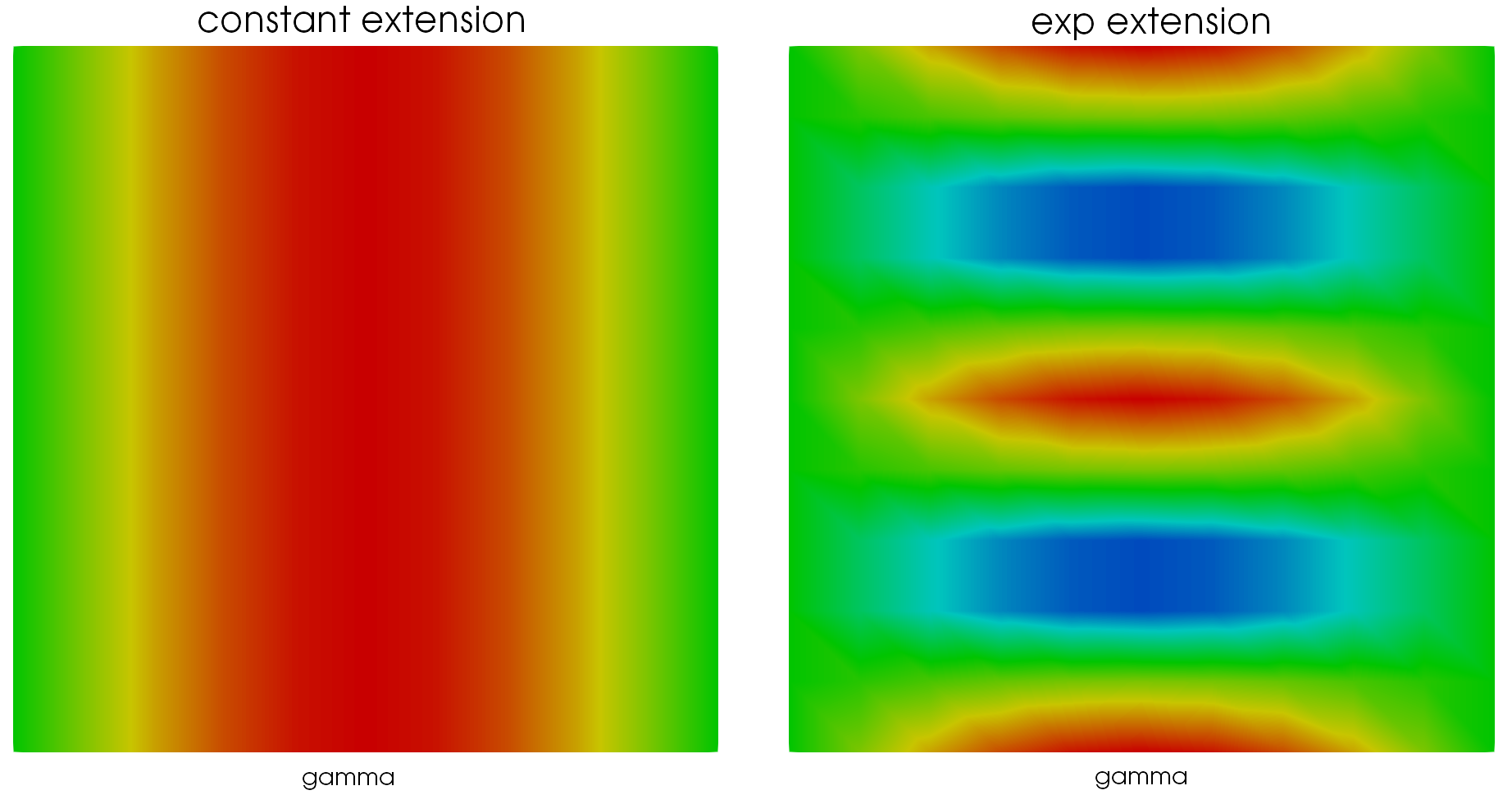
Extensions#

It is possible to extend a TermVector from a domain \(D\) to another one, say \(D_{ext}\). The extension of a function \(f\) is defined as following:

\[f_{ext}(M)=f(g(M)) \otimes h(M) \quad \forall M \in D_{ext}\]

where \(g\) is a map from \(D_{ext}\) to \(D\), \(h\) an additional function and \(\otimes\) a consistent operation between \(f\) and \(h\) (* by default).

As an example:

Real fsin(const Point& P,Parameters& pa = defaultParameters)
{return sin(pi_*P(1));}
Vector<Real> fmap(const Point& P,Parameters& pa = defaultParameters)
{return Point(P(1),0.);} // map omega-> sigma1
Complex fexp(const Point& P,Parameters& pa = defaultParameters)
{return exp(4*i_*pi_*P(2));}
...
Strings sidenames={"Gamma","","",""};
Mesh mr(Rectangle(_xmin=0, _xmax=1, _ymin=0, _ymax=1, _nnodes=11, _edge_names=sidenames), _shape=_triangle, _order=1, _generator=_structured);
Domain omega=mr.domain("Omega"),gamma=mr.domain("Gamma");
Space V(_domain=omega, _FE_type=Lagrange, _order=1, _name="V");
Unknown u(V, _name="u");
TermVector t(u,gamma,fsin, _name="t");  // nodal TermVector on side gamma
Function g(fmap), h(fexp);
TermVector extc=extension(t,g,omega,u);   // build constant extension (h=1)
TermVector exte=extension(t,g,omega,u,h); // build exp extension

Projections#

When a Projector is constructed (see Spaces and projections), the matrix \(\mathbb A\) and \(\mathbb B\) are computed and the matrix \(\mathbb A\) is factorized. So the projection of TermVector (consistent with the projector) can be computed:

TermVector B2(u2, omega, fx2, _name="B2"); // fx2 user function
TermVector B1=P2toP1(B2, u1);

By specifying the unknown u1 as second argument, the result B1 will have u1 as unknown. It is also possible to omit the unknown argument or to pass the TermVector result as argument:

TermVector B1=P2toP1(B2);
TermVector B1b;
P2toP1(B2, B1b);

When no unknown is given, XLiFE++ will choose the first unknown that has been defined on result space.

By using the projection function, the standard projections can be done without managing explicitely a Projector object:

TermVector B1=projection(B2, V1);

In that case the Projector object is constructed in the back and kept in memory.

Hint

Only single unknown TermVector can be projected. In case of multiple unknown TermVector, extract the part related to the unknown of interest before projection (see Restrictions).

About transient and eigen problems#

In order to write transient problems the easiest way possible (see Solving wave equation with Leap-frog scheme), the class TermVectors allows you to deal with a collection of TermVector. but there are a plenty of situations where it is friendly to use TermVectors, such as eigen problems for which you want to compute eigen vectors.

TermVectors tvs(20);
tvs(1)=...;
tvs(2)=...;
...

TermVectors can be constructed by giving its size and then, each TermVector of the collection can be accessed with the () operator (index numbering starting from 1).

An example with DtN map as transparent boundary condition#

The following example illustrates multiple uses of algebraic operators on TermMatrix.

...
// define spectral space to deal with DtN
Number N=10;
Space Sp(_domain=sigmaP, _basis=Function(cosny, params), _dim=N, _name="cos(n*pi*y)");
Unknown phiP(Sp, _name="phiP");
Complexes lambda(N);
for (Number n=0; n<N; n++) lambda[n]=sqrt(Complex(k*k-n*n*pi_*pi_/(h*h)));
// define TermMatrix with no DtN
BilinearForm auv=intg(omega, grad(u)|grad(v)) - k*k*intg(omega, u*v);
TermMatrix A(auv, _storage=csDual, _name="A");
// contruct DtN TermMatrix using matrix product
BilinearForm euv=intg(sigmaP, phiP*v), fuv=intg(sigmaP, u*phiP);
TermMatrix E(euv, _name="E"), F(fuv, _name="F");
TermMatrix L(phiP, sigmaP, lambda, _name="L"); // diagonal matrix
TermMatrix ELF=E*L*F;
TermMatrix A2=A-i_*ELF;

This DtN approach using product of matrices was the Melina approach. In XLiFE++, it is better to use TensorKernel approach. See Tensor kernels for more details.